Stable Isotopes and Diet Analysis: Insight into Trophic Level, and Geographical Origin and Location

Trevor Hum, Xavier Santerre, Kyle Vamvakas, Mathilde Wagner

Abstract

This paper delves into the details and applications of stable isotope and diet analysis. The report begins by giving a general overview of some key terms, ideas, and applications of stable isotopes and their use in research. It then follows with a comprehensive investigation of stable isotope analysis in terrestrial and marine animals, as well as C3, C4, and CAM plants. An emphasis is made on a few interesting studies that utilized stable isotope analysis to gather information on animal diets, trophic levels, and geographical origins. 

Stable Isotopes: A General Overview

What Are Isotopes?

While all atoms of the same element possess the same number of protons, it is possible to find variations in the mass number of some atoms of that element. This flexibility is explained by the fact that the number of neutrons in the nuclei of the atoms of an element is not consistent, as depicted in Fig. 1. These alternative forms of the same element are referred to as isotopes (“What Are Stable Isotopes?” | Stable Isotope Facility | University of Wyoming, n.d.).

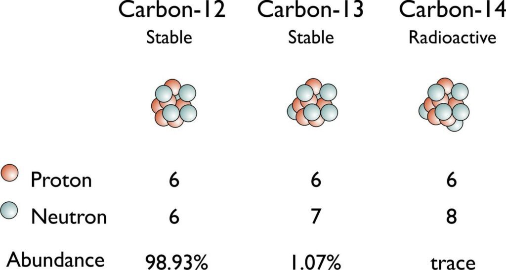
Isotopes can be differentiated in writing by their different atomic mass numbers, which corresponds to the sum of the number of protons and neutrons. For example, ¹⁴C and ¹²C differ by 2 neutrons, which can be respectively calculated by subtracting the atomic number from the atomic masses, since the number of protons does not vary. This would explain why one finds decimals when looking at the atomic mass numbers on the periodic table of elements. That is the average atomic mass, which must account for all the isotopes of each element, as well as each of their respective abundances. This is calculated in the following formula (“How To Find Atomic Mass and Number of Elements” | Periodic Table, 2020):

Average\space Atomic\space Mass=\textstyle\sum_{i=1}^n Mass_i  \sdot {\%Abundance_i\over 100}

(1)

While most isotopes express radioactive decay, some isotopes are said to be stable if they do not emit radiation and do not decay into other elements.

Among stable isotopes, one can further differentiate them by labelling them as heavy or light. Heavy stable isotopes have stronger attractive forces and bonds than their light counterparts, resulting in varying reaction rates in some important biological and environmental processes. This will lead to one finding differing ratios of heavy and light stable isotopes in various compounds of separate origins (Zimmo et al., 2012). The action of separately altering the levels of the abundances of the two different isotopes in a sample is a process known as fractionation. The relative abundances of the heavy and light stable isotopes, caused by fractionation, can often tell us something about the origin of the sample that is being analyzed.

Quantifying Isotopes

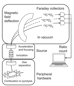
Before analyzing the ratios, one must first determine a way to obtain them from the sample in an accurate manner. The most common way of doing so is through thermal ionization mass spectrometry, or TIMS. In this process, the sample is weighed, turned to gas via combustion or pyrolysis, ionized and then accelerated through a magnetic field. This will cause the ions to separate depending on their mass, causing the heavy isotopes to land away from the light isotopes, as depicted in Fig. 2. Ensuring that no contamination occurs in this process is essential when working with small samples.

To begin comparing the ratios of the isotopes in different samples, a standard was established to have a baseline to compare to. For example, the international standard to compare deuterium, ²H, and hydrogen, ¹H, is the Vienna Standard Mean Ocean Water, with a ²H/¹H ratio of 0.00015575.  One can then use the following formula (Zimmo et al., 2012) with the established standards to interpret the ratio of isotopes from any given sample:

δX={R_{Sample}-R_{Standard}\over R_{Standard}} \sdot 1000

(2)

In this formula, X represents the heavy isotope, since R_Sample is, by convention, the ratio of the heavy isotope to the light isotope. The unit used to measure is parts per thousand, or per mil. Examples of applications and of case studies will be explored in Sections 2 and 3. However, the more general applications of this formula can be seen in the following subsection.

Applications of Stable Isotopes

As stated beforehand, many processes can lead to fractionation. The reason this is interesting is because it was discovered in the late 1970s that the isotopic ratio within foods will have a direct effect on the ratios expressed in the tissues of the consumer.

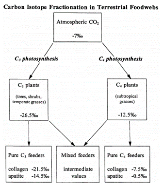
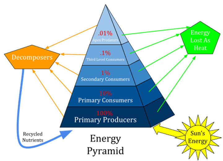
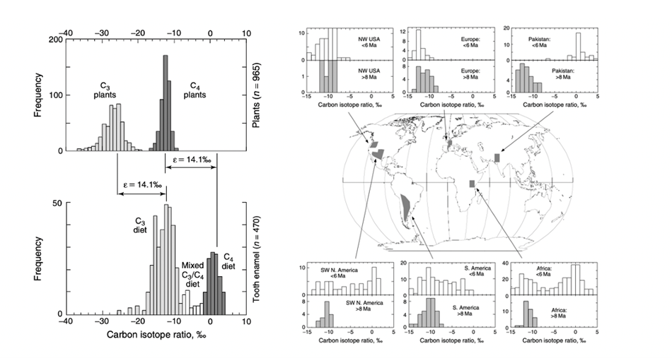
One key biological process that exhibits fractionation is photosynthesis. Depending on the pathway used, plants can achieve varying ratios of ¹³C to ¹²C. These two types of plants, labelled C4 and C3, as well as their photosynthetic pathways, will be elaborated on in detail later in the paper. Thus, if one wanted to determine what type of plant an animal was consuming, one can examine the ratio of the carbon isotopes in an animal’s tissues in order to determine if the animal’s diet was mainly based on C4 or C3 plants (Zimmo et al., 2012). This could also be useful in determining the geographical whereabouts of the animal, considering C4 plants are found mainly in warmer and drier climates. It was also determined that there was some correlation between the trophic level of an animal and the enrichment of ¹³C.

Another topic that became very important in reconstructing diet is the study of nitrogen isotopes ¹⁵N and ¹⁴N. As a result of comparing 𝛿¹⁵N among individuals of an ecosystem, it was determined that as a result of bioaccumulation and better retention of ¹⁵N, the 𝛿¹⁵N would increase by a value of around 3.4 % per trophic level. Thus, one can estimate the meat content in one’s diet, as well as the consumer’s trophic level. For example, if one finds a low 𝛿¹⁵N, one can conclude that the animal was low on the food chain, or perhaps even a vegan (Adams and Sterner, 2000). This can help researchers determine a lot about an ecosystem they are studying, as well as give even more information on the animal’s diet that perhaps, carbon isotopes alone could not.

Meanwhile, oxygen and strontium isotopes were gaining a lot of attention due to their ability to give researchers an idea of where certain animals originated from, rather than diet. Oxygen isotopes ¹⁶O and ¹⁸O are considered to obtain an idea of the geographical origin of an animal. Considering that evaporation is based on phase changes, which are based on energy, it is easy to see that fractionation can occur as water molecules with ¹⁶O will be easier to evaporate than ¹⁸O, leading to the enriching of ¹⁸O. Oxygen isotopes are introduced to the animal’s body via ingestion, generally by the water one drinks, be it tap water, or water in the wilderness.

Strontium isotopes ⁸⁷Sr and ⁸⁶Sr are especially important in determining one’s origins since each location seems to have a characteristic “fingerprint” 𝛿⁸⁷Sr. What is even more important is that, unlike nitrogen isotopes, ⁸⁷Sr will not get enriched as one increases in trophic levels. Thus, this distinct 𝛿⁸⁷Sr can be used very efficiently to determine the whereabouts of an animal (Tykot, 2004). These isotopes can be taken in by an animal in the water and food it consumes.

Thus, the idea of “you are what you eat” becomes very useful when studying animals via stable isotopes. Since bone collagen and carbonate require continuous upkeeping, taking a closer look at the isotopic ratios in these tissues can provide us with an idea of what kind of average diet an animal had throughout its lifetime. More specifically, studies found that the protein in one’s diet is responsible for bone collagen, while, on the other hand, the protein, fats, and carbohydrates from an animal’s meal will be used for the production of bone and tooth enamel apatite (Tykot, 2004). If one wishes to learn even more about an animal’s diet, whereabouts, and how it may have evolved overtime, one simply needs to examine the animal’s tooth enamel apatite, as well as their hair, and compare it to the bones.

Teeth form at various time periods in an individual’s life. Deciduous teeth are formed in utero, while one’s permanent teeth will form generally before puberty. However, since they do not require constant remodeling, their composition will remain the same since the time they were formed (Tykot, 2004). Therefore, examining these teeth’s isotope ratios can provide a researcher a great deal of information on an animal’s early life. More specifically, if one discovers a large discrepancy between the carbon isotope ratios of the tooth enamel and bone apatite, one can infer that there must have been a change in diet transitioning from the animal’s early to mid or late life. This can be due to a variety of factors, a common one being relocation. Furthermore, if the 𝛿¹⁸O varies from tooth to bone, the animal may have changed water source throughout its life, which is also indicative of relocation and movement. Likewise, comparing 𝛿⁸⁷Sr of both teeth and bone of an animal will be immediately apparent if this animal had moved or relocated since its childhood. This was essential when studying the Beaker People, who lived around 4 500 years ago. Using strontium isotopes, it was determined that they were very mobile. Also, in Teotihuacan, Mexico, it was determined that many people had originated from Monte Alban, and then later, moved to Teotihuacan, through analysis of the strontium isotopes in the teeth and bones (Tykot, 2004).

On the other hand, an animal’s hair is constantly synthesized. Thus, the content of an animal’s diet can be incorporated into the hair’s amino acids. An analysis of the isotopes in the hair can reveal the animal’s recent diet and can thus inform researchers of recent dietary changes when compared to the animal’s bones. An example of how this was applied is when a cold case in Salt Lake County, Utah made substantial strides in light of this new technology by comparing an unidentified victim’s hair’s oxygen isotopes to the ones found in tap water found across the United States (Brindley, 2008). As shown in in Fig. 4, the ratios of hydrogen and oxygen can vary wildly across even just a country, allowing police departments to analyze one’s hair to determine the recent general whereabouts of a victim or suspect.

Stable Isotope Analysis of Terrestrial Animals

Studying stable isotope ratios of terrestrial animals provides a lot of information about an individual. Isotopic signatures of terrestrial animals reflect the proportion of heavy to light isotopes of what they consumed, and a few included a discrimination factor (physiological processes they utilize in assimilating products). 

Stable isotope analysis is the technique we must use to examine the foraging ecology of extinct terrestrial animals.                             

Differences Between Carnivores and Omnivores

Isotopic Ratios

While stable isotope analysis already differentiates terrestrial and marine animals, this process also highlights differences between carnivores and herbivores.

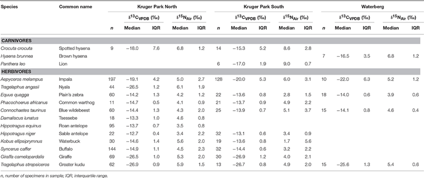
Generally, studies indicate that in herbivores, narrower isotopic niche breadths were observed compared to carnivore populations. For instance, a study by Daryl Codron et al. (“Within-Population Isotopic Niche Variability in Savanna Mammals”) investigates levels of carbon and nitrogen isotopic niche variation and niche partitioning within populations of species of carnivores and herbivores from the South African savannas. The same study also reveals lower levels of isotopic differentiation across individuals in herbivore species (Table 1 and Fig. 5).

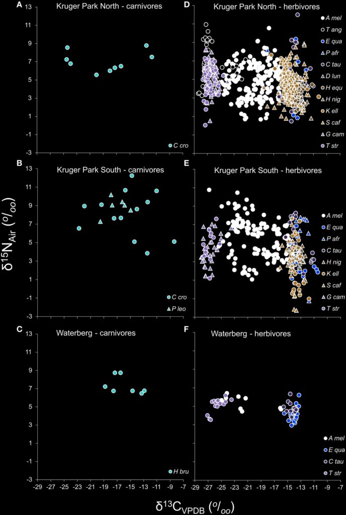
It has been observed that nitrogen isotope ratios are more enriched in terrestrial carnivorous mammals compared to herbivores. Specifically, terrestrial carnivores and herbivores have different mean δ¹⁵N values of +8.0 and +5.3 % (for bone collagen), respectively.

Furthermore, researchers (Ben-David and Flaherty, 2012) demonstrated that, for carnivores, lipid substance influences incorporation of carbon and nitrogen from dietary macronutrients. On the other hand, Florin et al. (2011) illustrated that, for herbivores, lipid content diets may be less important than protein quality and amount in determining discrimination values and incorporation rates.

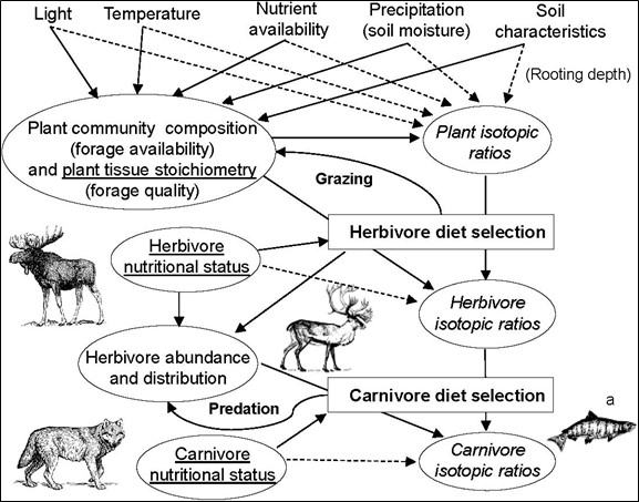
Factors of Differentiation of Isotopic Ratios (Environment/Diet)

Lots of interactions influence stable isotope ratios of terrestrial herbivores and carnivores, as illustrated in Fig. 6.

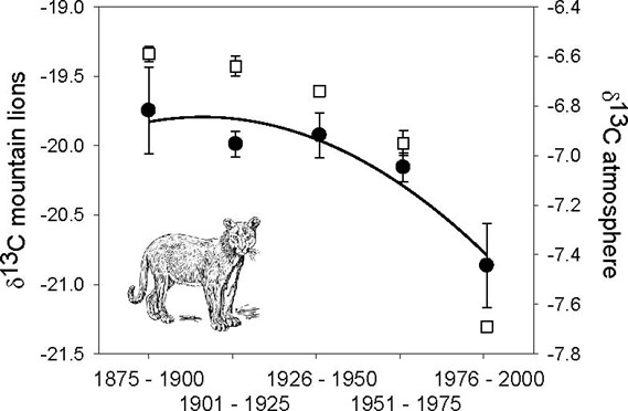
As shown above, temporal conditions have an importance in isoscapes (Lee et al., 2005, as cited in Ben-David and Flaherty, 2012). A study on mountain lions used museum specimen collected between 1893-1995 and found a temporal decrease in δ¹³ C values (in bone collagen).

While the decline of 1.2 % in mountain lion values could have been interpreted as a dietary change, the change was more likely caused by a depletion of atmospheric δ¹³ C values, which percolated through the food web.

Most importantly, as explained in Stable Isotopes: A General Overview, “diet and isotopes are interdependent in terrestrial animals, take for example insects; researchers Larsen et al. (2009) demonstrated that fungi, bacteria, and amino acids that have distinct isotopic signatures can be found in insects that consume them. Similarly, a study shows that gerbil’s tissues have different δ¹³ C values when fed a corn (C4) or wheat (C3) diet. Indeed, the gerbil’s isotopic composition shifted according to the food source (Tieszen et al., 1983). As a matter of fact, analysis uniquely of feces or gut content would give information of an animal’s diet during its recent past (few hours for insect, several days for terrestrial herbivorous mammals), while isotope analysis would be indicative of dietary carbon’s integration over a longer period.

Terrestrial Animal Trophic Levels

The relative simplicity of food chains within these systems means that variations within trophic levels are easily traced by using stable isotope analysis.

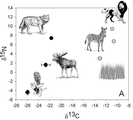
The degree of enrichment in ¹⁵N (depending on the diet of the terrestrial animals) differentiates from one trophic level to the next, determining the food chain (DeNiro and Epstein, 1981, as cited in Ben-David and Flaherty, 2012).

Migration of Terrestrial Animals

Several investigations of migration of terrestrial animals based on δ D values in keratin were led by Chamberlain et al. (1997) and Hobson and Wassenaar (1997). For instance, to identify the migration and movement of mastodons (Mammut) and mammoths (Mammuthus) in Florida during the Pleistocene, Hoppe and Koch (2007) used the analysis of ⁸⁷Sr: ⁸⁶Sr isotopes in fossil tooth enamel. Using this technique, they could associate long- range movements to mastodons, and found out mammoths traveled relatively short distances.

To end this subsection, terrestrial animals have stable isotope ratios that differ greatly. Major differences are observed between carnivores and herbivores, reflecting their diet, and thus the ingestion of different nutrients. To illustrate these remarks, an example for a terrestrial herbivore and a terrestrial carnivore are discussed below.

Detailed Examples

A Terrestrial Herbivorous Animal: The Elephant

The elephant is the largest living terrestrial animal. It is herbivorous, feeding on a large variety of grasses, creepers and herbs. The larger, L. Africana, is the savanna elephant and it is found in East and South Africa.

By analyzing the stable isotopes in tooth enamel or collagen in modern elephants (Elephas in Asia and Loxodonta in Africa), scientists (Sukumar and Ramesh, 1992) were able to determine their diet. They could also evaluate the diet of elephants that are no longer living by using fossils! Indeed, as tooth enamel is resistant to isotopic exchange, it can be a very useful tool to study these extinct elephant species and their habitats, regions, and diet (Fig. 10).

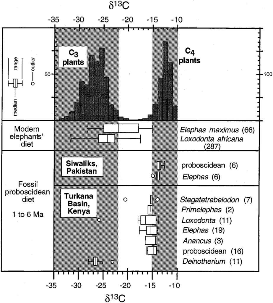
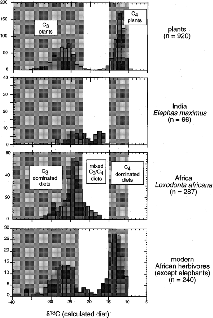
As illustrated above, the diet of modern elephants from Africa and Asia is C₃ dominated (δ¹³C diet  < -23‰), although some samples reveal a mixed C₃/C₄ diet (Fig. 11.). The δ¹³C values in collagen revealed that more carbon was incorporated from C3 plants, presumably because of their higher protein contribution.

This knowledge of the diet composition also gives information about the living region of the elephant species. For instance, elephants living in the montane forest in Kenya are more depleted in ¹³C than those from the savanna region, but not as depleted as elephants from the primary rain forest.

A Terrestrial Carnivore: The American Marten

Martens (Fig. 12.) are a carnivorous terrestrial mammal species.

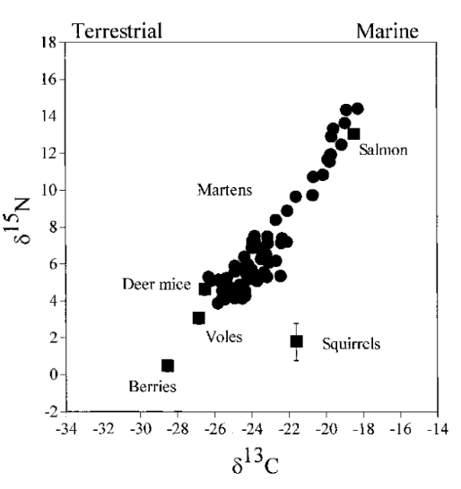
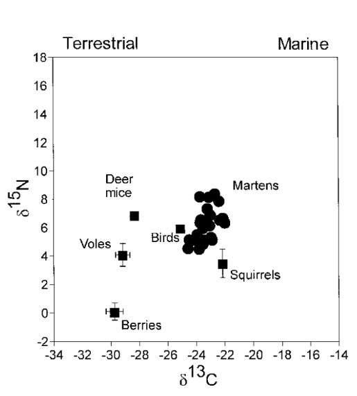
A study by Ben-David and colleagues in 1997 (“Annual and seasonal changes in diets of martens”) determined the diet source for each marten based on the combined values of δ¹³C and δ¹⁵N, in correlation with seasonal changes. What was also observed is the change of isotopic ratios of martens between different seasons (Fig. 13. and 14), as representative of abundance of the seasonal availability of salmon, birds and berries.

In autumn, diets of martens showed high variability in composition (Fig. 13.). Indeed, some martens fed mostly on salmon carcasses (more than 35 % of diet), and others relied mainly on small rodents (more than 35 % of diet). By using stable isotope ratios, we could demonstrate that, for example, in autumn during years of low abundance of rodents, martens’ diet is highly composed of salmon, martens, thus changing their foraging strategies. In the summer, the average of berries, on which martens rely, increases, and this change of diet composition due to this increase of berry consumption correlates with Fig. 14., compared to Fig. 13..

Stable Isotope Analysis of Marine Animals

There has been a great deal of success in analyzing stable isotopes to determine trophic level and dietary information of marine animals. Scientists have been able to compare stable isotope data between animals currently occupying a territory and animals that once occupied it. This has allowed scientists to see if a species is subjected to any changes in their diet over a period of time. A popular method to accomplish this is to gather stable isotope information from the teeth of marine animals. There are two noteworthy studies which highlight the use of stable isotope analysis in marine animal teeth. The first paper (Walker et al., 1999) compares stable isotope findings of bottlenose dolphins from different periods of time. The second paper (Hobson and Sease, 1998) shows why it is crucial to analyze stable isotopes of individual tooth annuli to get a more detailed account for variations of isotopic numbers.

“The Diets of Modern and Historic Bottlenose Dolphin Populations Reflected Through Stable Isotopes” by Walker et al. (1999) is a unique paper. Stable isotope composition in the teeth of bottlenose dolphin was analyzed in populations over an extended period of time. From the 1880s to 1920s to 1980s, the diet of northwest Atlantic bottlenose dolphins was thought to have changed because of chemical pollution and overfishing of their prey. Thus, the composition of carbon and nitrogen stable isotopes in the teeth of the three dolphin populations were compared to determine if their diet had change over that century.

The results, which are documented in Table 2, show no statistically significant difference between the isotopic compositions of ¹³C and ¹⁵N between the populations. Referencing the first section of the report, 𝛿¹³C and 𝛿 ¹⁵N dental signatures across the three populations are calculated using the following formula (Zimmo et al., 2012) that was mentioned in Stable Isotopes: A General Overview:

δX={R_{Sample}-R_{Standard}\over R_{Standard}}   \sdot1000

(3) 

The calculation expresses the relative abundance of an isotope of an element from a sample to the standard abundance of that isotope. Comparing the mean 𝛿¹³C and 𝛿¹⁵N dental signatures across the three populations, there is a slight trend in the enrichment of the isotopic compositions from the 1880s dolphins to the 1920s dolphins, and from the 1920s dolphins to the 1980s dolphins. Fig. 15. shows this data plotted on a graph.

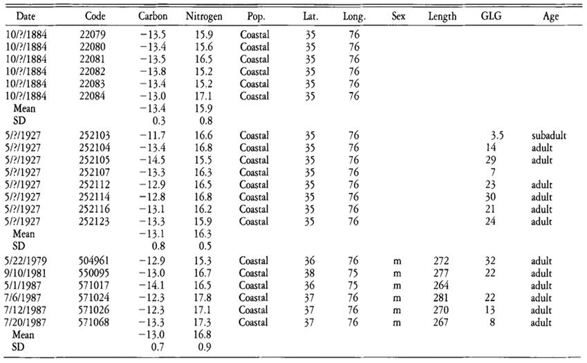
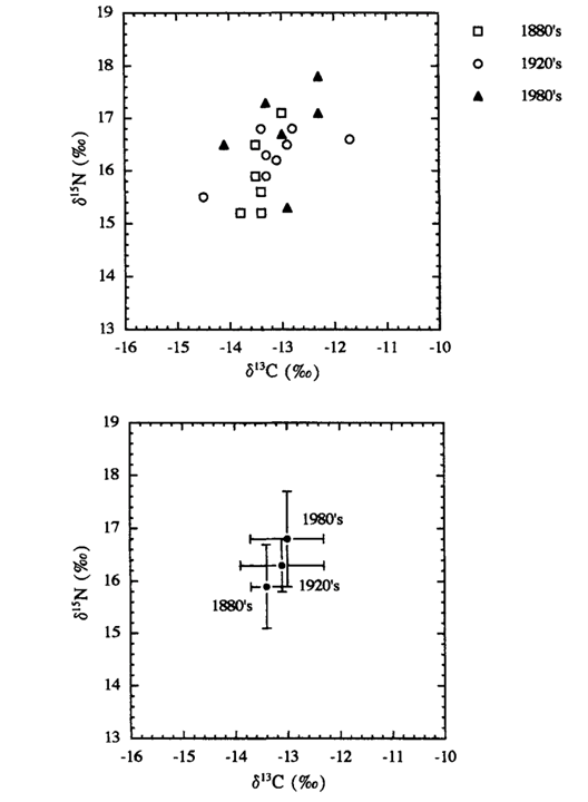
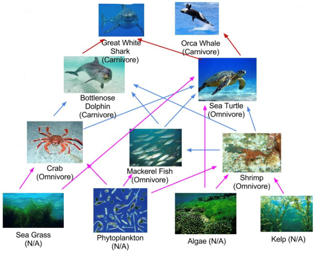
The findings suggest the diets of northwest Atlantic bottlenose dolphins were similar throughout those three decades. What is even more interesting is that gut contents of the dolphins from all three decades were also documented. From the 1880s, common gurnard was found in the guts of two dolphins. In the 1920s, fishermen documented that the dolphins mainly consumed weakfish; and the dolphins from the 1980s mainly consumed sciaenid fish. The common characteristic among the fish the dolphin populations consumed is they are benthic feeders. These benthic feeding fish primarily consume crustaceans, like crabs and shrimp, as well as other smaller fish. This is why the 𝛿¹³C and 𝛿¹⁵N dental signatures of the dolphins across the different time periods are so similar. Relating this information to the food web of the bottlenose dolphin (Fig. 16.), it suggests the northwest Atlantic bottlenose dolphin has remained at the same trophic level over the course of those 100 years. They all consume fish that were primary consumers, and as a result, all have similar 𝛿¹³C and 𝛿¹⁵N dental signatures. If there would have been a statistically significant increase or decrease of 𝛿¹³C and 𝛿¹⁵N between the dolphin populations, this may have suggested the dolphins changed trophic level. It may have also suggested human activity was affecting the abundance of ¹³C and ¹⁵N in the region. However, this was not the case. The dolphins remained at the same trophic level and did not suffer any significant consequences as a result of chemical pollution and overfishing.

The second study, “Stable Isotope Analyses of Tooth Annuli Reveal Temporal Dietary Records: An Example Using Steller Sea Lions” by Hobson and Sease (1998), uses stable isotope analysis of teeth as well. However, the technique applied is slightly more sophisticated than the one used in Walker et al.’s research (1999). The technique applied analyses stable isotopes in individual tooth annuli, rather than only considering the mean 𝛿¹³C and 𝛿¹⁵N dental signatures of all the teeth. This method not only allows scientists to gather information on the diet and trophic level of an animal, but also provides information on an animal’s diet over the course of their life. 

In this study, the teeth of Steller sea lions of different ages, spanning different time periods, were examined. To compare data from species of different trophic levels, the teeth of one fur seal and one elephant seal were also examined. All the animals were from regions around Alaska, which is illustrated in Fig. 17..

The results of the study were quite surprising (Table 3 and Fig. 18.). For the Steller sea lions, 𝛿¹³C and 𝛿¹⁵N dental signatures varied considerably among the annuli; however, this was not case for the fur seal and elephant seal.

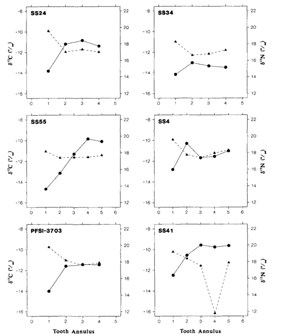
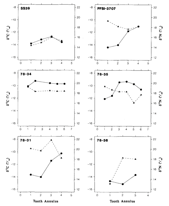
From these results, it is important to emphasize why annuli sampling is more indicative of an animal’s diet compared to taking an average of all the annuli. For example, if an average of 𝛿¹³C and 𝛿¹⁵N dental signatures are taken from the annuli of a young sea lion, it will give a more enriched 𝛿¹⁵N value because it has recently stopped consuming its mother’s milk, which is rich in ¹⁵N. However, the average 𝛿¹⁵N value would be an overestimate of the abundance of ¹⁵N present in the young sea lion’s current diet. There is a similar issue when taking the average 𝛿¹³C and 𝛿 ¹⁵N dental signatures of all tooth annuli of older sea lions as well, if for example, they change trophic level or migrate to a different location with different ¹³C and ¹⁵N abundances (Hobson and Sease, 1998).

For many of the Steller sea lions, the year one 𝛿¹⁵N values were more enriched than the subsequent years, and these enriched values were also observed in the first tooth annulus when compared to the other annuli. The reason behind the enriched ¹⁵N diet observed in the early life of the sea lions has to do with their source of nutrition when they are a pup, the mother’s milk. The milk is more enriched in ¹⁵N compared to the prey adult sea lions consume. The reason for the mother’s milk being more enriched in ¹⁵N is due to trophic enrichment. The prey the mother consumes is more enriched in ¹⁵N than the food the prey had consumed, and so forth. Subsequently, the milk will be more enriched in ¹⁵N than the prey adult sea lions consume, which accounts for the drop off between first year and subsequent year 𝛿 ¹⁵N values in the annuli.

Comparing the mean 𝛿 ¹⁵N values between the Steller sea lions, the elephant seal, and the fur seal gives insight into their respective trophic levels. The data Hobson and Sease present suggests that adult sea lions consumed prey with an average 𝛿¹⁵N value of about 16‰, whereas the elephant seal consumed prey with an average 𝛿¹⁵N value of about 14.8‰, and an average 𝛿 ¹⁵N value of about 13.1‰ for the fur seal. From this data, it is evident the sea lions were consuming at the highest trophic level, followed by the elephant seal, and then followed by the fur seal (Hobson and Sease, 1998).

Focusing specifically on the stable isotope analysis of the sea lions, there has been a slight increase in their trophic level from 1943 to 1991. Taking a look at the mean 𝛿¹⁵N values of the sea lions after year one, there was an increase from about 17‰ in 1943 to 19‰ in 1991, with a high correlation observed in the sea lions between those two years. This information could lead scientists to uncover a lot more information about food webs in the Alaskan region (Hobson and Sease, 1998). The trophic level increase in sea lions suggests changes had to have happened at the lower trophic levels. There are many possibilities that may account for the change. One particularly interesting possibility is that other species of marine animals of lower trophic levels may have migrated over the 50-year period. Of course, there are many other possibilities to account for this change, but that is just one to keep in mind. 

Even more fascinating, the application of stable isotope analysis highlighted in Walker et al.’s study (1999) and Hobson and Sease’s (1998) is just one of its many applications. For instance, instead of comparing the same species over a period of time, scientists use stable isotope analysis to compare ¹³C and ¹⁵N abundance in neighboring regions. Bringing it back to Hobson and Sease’s research, two completely different regions, which both have sea lions, could have their stable isotope analyses compared to one another. This allows for much more than just determining their diet and trophic level, but also allows scientist to determine if external factors caused by humans affects the entire region’s stable isotope abundance. With this information, more data can be compiled to know which human activities affect stable isotope abundance in marine food webs and which do not.

C3, C4 and CAM Plants

There are three different types of photosynthetic pathways, and therefore, three different types of autotroph plants in the biodiversity of Earth: C3 plants, C4 plants and CAM (crassulacean acid metabolism) plants (Ehleringer and Cerling, 2002). As explained in the section Stable Isotopes: A General Overview of this paper, the isotope composition in C3, C4 and CAM plants influences the distribution of isotopes present in the tissues of herbivores and carnivores, due to the fact that plants are at one of the lowest trophic levels in ecosystems. In other words, herbivores and omnivores consume C3, C4 or CAM plants, each of which have a different isotopic composition. This composition is directly linked to the composition of isotopes in their tissues and cell. They can then be eaten by a carnivore or omnivore species, and the isotopic composition of the plant will be reflected in that animal. Therefore, the lower the species is on the trophic level, the bigger the impact it can have on all the other species that are directly or indirectly linked to it (Fig. 19.).

Photosynthesis

There are two main processes that most beings on Earth use to produce ATP (energy for cells): cellular respiration and the light reactions of photosynthesis. Photosynthesis is a process used by autotroph species – species that convert non-organic substance into energy, without the need of another species (BD Editors, “Photosynthesis”), mainly done by plants. This process occurs, for plants, in the chloroplast, an organelle present in their cells (Fig. 20).

The way plants produce their energy is simplified by the equation:

We will mainly focus on the part of the reaction mechanism which represents the photosynthesis process (the second reaction mechanism accounts for cellular respiration in plants). There are two main phases in photosynthesis: the light reactions and the Calvin cycle (Fig. 21).

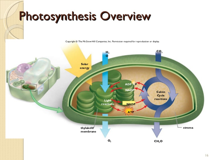
We will not get into the details of photosynthesis, but simply explained, H₂O is split and releases 2 electrons and O_2. This last component will be released in the atmosphere. During that time, photon particles hit the photosystems — proteins of the thylakoid membrane (Yahia et al., 2019) — which excites the electrons released by the water. These electrons then pass through a series of reactions to finally be converted to ATP and NADPH + H⁺. NADPH stands for nicotinamide adenine dinucleotide phosphate, which is a compound that helps in the reaction of an enzyme as a catalyst (“NADPH” | National Center for Biotechnology Information, n.d.). This series of reactions engaged by photons and H₂O are called light reactions. The ATP and NADPH + H+ then enters the Calvin cycle where they, and other compounds, will interact directly or indirectly with CO₂ in a cycle of reactions, to create CH₂O — carbohydrate — and ATP (Fig. 22). The carbohydrate will then be transformed into ATP in cellular respiration.

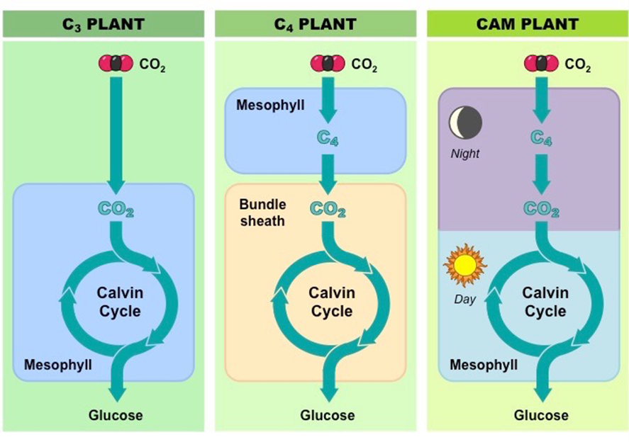
C3 Plants

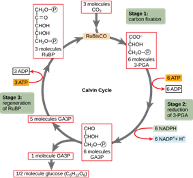
C3 plants are the most ancient plants of the three types mentioned above. These plants frequently use photorespiration. In every plant, the CO₂ is added to the diphosphate thanks the Rubisco enzyme in the first step of the Calvin cycle (Fig. 22). Plants that utilize this process are called C3 plants since the product of this addition is 3-phosphoglycerate, which has three carbons. Rice, soybeans, potatoes and sugar beets are some examples of C3 plants (Jenkins, 2014). CO₂ enters the plant’s cell through the stomata, which are pores in the plant’s epidermis, located on the leaves, while O₂ and water vapor also use this pathway to exit the cell (Ask Nature Team, “Leaves Adapt to Dry, Hot Conditions). Since water vapor exits through these pores, plants have developed a mechanism that allows them to close their stomata when the temperature rises, preventing them from losing too much H₂O. The problem is that when the only pathway in and out of the leaf is closed, CO₂ cannot enter, and the photosynthetic process is slowed down (Ask Nature Team, “Leaves Adapt to Dry, Hot Conditions”). Moreover, the Rubisco enzyme is also able to catalyze the fixation of O₂ instead of CO₂ in the first reaction, meaning the two compounds can both be fixed to the same active site of the enzyme. Therefore, when the amount of CO₂ drops, the reaction continues, but uses O₂ instead of CO₂, which results in the creation of CO₂ and the loss of ATP. This unfavorable process is photorespiration (Fig. 23). Scientifics do not understand why nature has not created Rubisco in a way that it can only react with CO₂, but the main hypothesis is that when it first appeared, the atmosphere was less concentrated in oxygen than it is today, making the photorespiration almost impossible (Erb and Zarzycki, 2018). However, even though photorespiration is considered inefficient because it stops the production of O₂ and glucose, and creates CO_2, this reaction helps plants protect themselves against the sun when the temperature is too high.

C4 plants

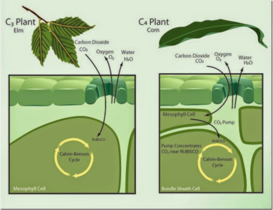
C4 plants emerged later. These plants developed a special mechanism that allows them to photosynthesize on hot and sunny days. Corn, sugarcane and switchgrass are some examples of this type of plants (“C3 and C4 photosynthesis” | InTeGrate | Carleton University, n.d.). They inherited their name from the fact that these plants attach the CO₂ to a 4-carbon compound – oxaloacetate –in an additional step of photosynthesis. In fact, C4 plants have a different leaf physiology than C3 plants, which allows them to do photosynthesis in conditions where the Rubisco is not capable of being utilized (Erb and Zarzycki, 2018). C4 leaves are made of mesophyll cells and bundle-sheath cells, in comparison to C3 leaves, which are made of mesophyll cells only (Fig. 24). In this specific type of plants, the CO₂ enters the leaves through the stomata to be fixed by the PEP carboxylase – also known as phosphoenolpyruvate carboxylase, this compound is an enzyme unique to C4 and CAM plants (“PEP carboxylase” | Biology Online Dictionary, n.d.) – to phosphoenolpyruvate, creating the four-carbon compound, oxaloacetate. This fourth carbonated compound, created in the mesophyll cells, is then transported to the bundle-sheath cell where the bicarbonate will be released and stored for the Rubisco to use, in order to begin the Calvin cycle (Fig. 24). This process also regenerates the PEP carboxylase, allowing it to start the same process over and over again. What is more, PEP carboxylate is 10 times more attracted to CO₂ then Rubisco is, making it a significant advantage in hot conditions, when the stomata are closed (Erb and Zarzycki, 2018). Moreover, it has no attraction to dioxygen, almost eliminating the photorespiration in C4 plants, and thus reducing what humans have defined as energy waste.

CAM Plants

Over time, another type of plant using a different photosynthetic adaptation emerged. These plants also developed a way to reduce the use of the photorespiration process during hot days: CAM plants (BD Editors, “CAM Plants”). These plants usually have big thick leaves that can store water, like pineapples and many varieties of cactus. CAM plants and C4 plants work in a similar way, the difference being that CAM plants collect CO₂ at night and transform it to different varieties of organic acids, which are stored and will be transformed back to CO₂ the following day when the sun is not as strong (BD Editors, “CAM Plants”). This specific storage mechanism is called the crassulacean acid metabolism since it produces many different organic acids. CAM plants are the only plants that open and close their stomata in a reversed way; closed during the day and open at night (BD Editors, “CAM Plants”).

Isotopes

Researchers have discovered that C3 plants, when collecting CO₂ with Rubisco, tend to prefer ¹²C from ¹⁴C in the CO₂. The C4 and CAM plants, on the other hand, also tend to prefer the lighter isotope, but less than the C3 plants. Therefore, it is possible to use this difference in concentration of ¹²C and ¹⁴C in an animal’s tissues to analyze its diet and see what type of plants it prefers (Ben-David and Flaherty, 2012). C4and CAM plants are also mostly located in warm countries due to their immunity to high temperature. Therefore, scientists can use the concentration of ¹²C and ¹⁴C isotopes to determine if a species is feeding directly or indirectly on plants, has migrated from a cold place to a hot place, or vice versa (Ben-David and Flaherty, 2012).

Climate Change

It is well known that climate change is happening as we speak, affecting not only humans but also other organisms like plants. Climate change is mostly caused by the rising concentration of CO₂ in the air. The high concentration of this gas could be a good thing for C3 plants who use photorespiration (Hirst, 2019). However, the temperature is also rising, causing the stomata to close even more and making water scarcer. On the other hand, C4 and CAM plants are immune to these changes since their photosynthesis mechanism functions in these tougher conditions. Even though scientists know these facts, they are worried about the long-term effect climate change could have on the distribution of these plants on Earth, and therefore, affecting many diets (Hirst, 2019)

Conclusion

Stable isotopes are very useful tools in studying ecosystems and the animals that reside within them. Their diversity and the various methods of fractionation can thus allow researchers to use them in a variety of experiments to reconstruct diet, establish trophic levels, and determine a geographical origin for modern and prehistoric animals. Within the terrestrial animal ecosystems, several differences between carnivores and herbivores are noticeable when comparing their isotopic ratios.

The same information could be learnt through stable isotope analysis of marine animals. This was emphasized by comparing stable isotope date in northwest Atlantic bottlenose dolphins over a 100-year period. Contrary to what the researchers were expecting, the dolphins did not see a change in their trophic level due to pollution and overfishing. Additionally, the method allows scientists to compare trophic levels of different species throughout a region, highlighted in the stable isotope analysis of Steller sea lions, the elephant seal, and the fur seal.

Stable isotope analysis is also a useful tool to use on plants. Plants are located on one of the lowest trophic levels, meaning their isotope composition impacts a lot species in their ecosystem. Since they are autotrophs, they use photosynthesis to produce their energy. Over time, three types of autotroph plants emerged, all having a different preference for different stable isotopes of carbon present in the CO₂ they consume. Using this knowledge, scientists may discover which type of plants an animal consumes, emphasizing once again the significance of stable isotope analysis.

References

(RIPE), R. I. P. E. (2020, 18 Mar 2020). The difference between C3 and C4 plants. Retrieved from https://ripe.illinois.edu/blog/difference-between-c3-and-c4-plants

Adams, T., & Sterner, R. (2000). The Effect of Dietary Nitrogen Content on Trophic Level 15N Enrichment. Limnology and Oceanography – LIMNOL OCEANOGR, 45, 601-607. doi:10.4319/lo.2000.45.3.0601

Aryal, S. (2020, 19 Apr 2021). Chloroplasts- Definition, Structure, Functions and Diagram. Retrieved from https://microbenotes.com/chloroplasts-structure-and-functions/

Ben-David, M., & Flaherty, E. A. (2012). Stable isotopes in mammalian research: a beginner’s guide. Journal of Mammalogy, 93(2), 312-328. doi:10.1644/11-mamm-s-166.1

Ben-David, M., Flynn, R., & Schell, D. (1997). Annual and seasonal changes in diets of martens: Evidence from stable isotope analysis. Oecologia, 111, 280-291. doi:10.1007/s004420050236

Ben-David, M., Shochat, E., & Adams, L. G. (2001). Utility of stable isotope analysis in studying foraging ecology of herbivores: Examples from moose and caribou. Alces, 37(2), 421-434. Retrieved from http://pubs.er.usgs.gov/publication/1013434

BioNinja. (n.d.). C3, C4 and CAM Plants. Retrieved from https://ib.bioninja.com.au/higher-level/topic-8-metabolism-cell/untitled-2/c3-c4-and-cam-plants.html

Boundless, G. M. a. (n.d.). The Calvin Cycle. In Microbiology (Boundless) Retrieved from https://bio.libretexts.org/@go/page/9006

Brindley, L. (2008). Your hair knows where you’ve been. Retrieved from https://www.chemistryworld.com/news/your-hair-knows-where-youve-been/3004358.article

Cerling, T. E., Harris, J. M., & Leakey, M. G. (1999). Browsing and grazing in elephants: the isotope record of modern and fossil proboscideans. Oecologia, 120(3), 364-374. doi:10.1007/s004420050869

Chamberlain, C. P., Blum, J. D., Holmes, R. T., Feng, X., Sherry, T. W., & Graves, G. R. (1996). The use of isotope tracers for identifying populations of migratory birds. Oecologia, 109(1), 132-141. doi:10.1007/s004420050067

Codron, D., Codron, J., Sponheimer, M., & Clauss, M. (2016). Within-Population Isotopic Niche Variability in Savanna Mammals: Disparity between Carnivores and Herbivores. Frontiers in Ecology and Evolution, 4(15). doi:10.3389/fevo.2016.00015

Conservancy, T. N. (2020, 16 Jul 2020). African Bush Elephant. Retrieved from https://www.nature.org/en-us/get-involved/how-to-help/animals-we-protect/african-bush-elephant/

Darcy, P. (n.d.). American Marten. In. Getty Images. Retrieved from https://www.gettyimages.fi/detail/photo/pine-marten-royalty-free-image/1073121342?adppopup=true

Deniro, M. J., & Epstein, S. (1981). Influence of diet on the distribution of nitrogen isotopes in animals. Geochimica et Cosmochimica Acta, 45(3), 341-351. doi:10.1016/0016-7037(81)90244-1

Dictionary, B. O. (Ed.) (n.d.). PEP carboxylase. In. Biology Online Dictionary. Retrieved from https://www.biologyonline.com/dictionary/pep-carboxylase

Editors, B. (Ed.) (2017). Photosynthesis. In. Biology Dictionary (online). Retrieved from https://biologydictionary.net/photosynthesis/#:~:text=July%2030%2C%202017-,Photosynthesis%20Definition,the%20bonds%20of%20glucose%20molecules.&text=These%20two%20energy%2Dstoring%20cofactors,carbon%20dioxide%20(CO2

Editors, B. (Ed.) (2019a). Trophic Level. In. Biology Dictionary (online). Retrieved from https://biologydictionary.net/trophic-level/

Editors, B. (Ed.) (2019b). CAM Plants. In. Biology Dictionary (online). Retrieved from https://biologydictionary.net/cam-plants/

Ehleringer, J., & Cerling, T. E. (2002). The Earth system: biological and ecological dimensions of global environmental change. In H. A. Mooney & J. G. Canadell (Eds.), Encyclopedia of Global Environmental Change (2 ed., pp. 186–190). Salt Lake City John Wiley and Sons.

Erb, T. J., & Zarzycki, J. (2018). A short history of RubisCO: the rise and fall (?) of Nature’s predominant CO2 fixing enzyme. Food biotechnology • Plant biotechnology, 49, 100-107. doi:10.1016/j.copbio.2017.07.017

Florin, S. T., Felicetti, L. A., & Robbins, C. T. (2011). The biological basis for understanding and predicting dietary-induced variation in nitrogen and sulphur isotope ratio discrimination. Functional Ecology, 25(3), 519-526. doi:https://doi.org/10.1111/j.1365-2435.2010.01799.x

Ford, E. (2013). Bottlenose Dolphin Food Web. Retrieved from http://www.thinglink.com/scene/378591197637115904

Hirst, K. K. (2019). Adaptations to Climate Change in C3, C4, and CAM Plants. Retrieved from https://www.thoughtco.com/c3-c4-cam-plants-processes-172693

Hobson, K. A., & Sease, J. L. (1998). STABLE ISOTOPE ANALYSES OF TOOTH ANNULI REVEAL TEMPORAL DIETARY RECORDS: AN EXAMPLE USING STELLER SEA LIONS. Marine Mammal Science, 14(1), 116-129. doi:https://doi.org/10.1111/j.1748-7692.1998.tb00694.x

Hobson, K. A., & Wassenaar, L. I. (1996). Linking breeding and wintering grounds of neotropical migrant songbirds using stable hydrogen isotopic analysis of feathers. Oecologia, 109(1), 142-148. doi:10.1007/s004420050068

Hoppe, K. A., & Koch, P. L. (2007). Reconstructing the migration patterns of late Pleistocene mammals from northern Florida, USA. Quaternary Research, 68(3), 347-352. doi:10.1016/j.yqres.2007.08.001

Information, N. C. f. B. (n.d.). PubChem Compound Summary for CID 5884, NADPH. In: NADPH. Retrieved from https://pubchem.ncbi.nlm.nih.gov/compound/5884

InteGrate. (n.d.). C3 and C4 photosynthesis. In: Carleton University. Retrieved from https://serc.carleton.edu/integrate/teaching_materials/food_supply/student_materials/1167

Jenkins, B. M. (2014). Global Agriculture: Industrial Feedstocks for Energy and Materials. In N. K. Van Alfen (Ed.), Encyclopedia of Agriculture and Food Systems (pp. 461-498). Oxford: Academic Press. Retrieved from https://www.sciencedirect.com/science/article/pii/B978044452512300156X

Larsen, T., Taylor, D. L., Leigh, M. B., & O’Brien, D. M. (2009). Stable isotope fingerprinting: a novel method for identifying plant, fungal, or bacterial origins of amino acids. Ecology, 90(12), 3526-3535. doi:https://doi.org/10.1890/08-1695.1

periodictable.me. (2020). How To Find Atomic Mass and Number of Elements. Retrieved from https://periodictable.me/tag/how-to-calculate-atomic-mass-of-isotopes/

Price, J. (n.d.). Carbon Isotopes. In. Pinterest. Retrieved from https://www.pinterest.ca/pin/405886985142270151/

Purdon, R. (2013). Simplified photorespiration and Calvin cycle. In Simplified_photorespiration_diagram.jpg (Ed.). Wikimedia Commons. Retrieved from https://en.wikipedia.org/wiki/Photorespiration#/media/File:Simplified_photorespiration_diagram.svg

S., Z., Blanco, J., & Nebel, S. (2012). The Use of Stable Isotopes in the Study of Animal Migration. Nature Education Knowledge, 3(12), 3. Retrieved from https://www.nature.com/scitable/knowledge/library/the-use-of-stable-isotopes-in-the-96648168/

Sang Heon, L., Donald, M. S., Trent, L. M., & Richardson, W. J. (2005). Regional and seasonal feeding by bowhead whales Balaena mysticetus as indicated by stable isotope ratios. Marine Ecology Progress Series, 285, 271-287. Retrieved from https://www.int-res.com/abstracts/meps/v285/p271-287/

Slideshare. (2011). Photosynthesis/Cell Resp. In. Slideshare. Retrieved from https://www.slideshare.net/coreylellison/photosynthesiscell-resp

Sukumar, R., & Ramesh, R. (1992). Stable carbon isotope ratios in Asian elephant collagen: implications for dietary studies. Oecologia, 91(4), 536-539. doi:10.1007/bf00650328

Team, A. N. (2017). Leaves Adapt to Dry, Hot Conditions. Retrieved from https://asknature.org/strategy/leaves-adapt-to-dry-hot-conditions/

Tieszen, L. L., Boutton, T. W., Tesdahl, K. G., & Slade, N. A. (1983). Fractionation and turnover of stable carbon isotopes in animal tissues: Implications for δ(13)C analysis of diet. Oecologia, 57(1-2), 32-37. doi:10.1007/bf00379558

Tikot, R. H. (2004). Stable isotopes and diet: You are what you eat. 154, 133-144.

Walker, J. L., Potter, C., & Macko, S. (1999). THE DIETS OF MODERN AND HISTORIC BOTTLENOSE DOLPHIN POPULATIONS REFLECTED THROUGH STABLE ISOTOPES. Marine Mammal Science, 15, 335-350.

Wyoming, U. o. (n.d.). What are Stable Isotopes? Retrieved from http://www.uwyo.edu/sif/stable-isotopes/what-are-stable-isotopes.html

Yahia, E. M., Carrillo-López, A., Barrera, G. M., Suzán-Azpiri, H., & Bolaños, M. Q. (2019). Chapter 3 – Photosynthesis. In E. M. Yahia (Ed.), Postharvest Physiology and Biochemistry of Fruits and Vegetables (pp. 47-72): Woodhead Publishing. Retrieved from https://www.sciencedirect.com/science/article/pii/B9780128132784000038