Quantifying Skin Patterns: Mathematical Interpretations of Camouflaging Techniques in Animals
Christopher Coluni, John Eric Hamilton, Olivia Lopardo, Olivier Morin
Abstract
The question whether a relationship between mathematics and biology exists has always been up for debate. The reason for such skepticism lies in the obvious complexity within living organisms and the amount of variability. Biologists have a certain level of distrust towards mathematical interpretations as they tend to oversimplify the experimental model. However, the mathematical strategy of reductionism is an extremely powerful tool and has helped biologists in the understanding of many scientific phenomena (Herrero, 2007). By interpreting biological mechanisms as collections of smaller elements, each contributing module can be studied in greater detail. Mathematical models can then be established for each of these smaller ingredients, resulting in much more elaborate understanding of the natural mechanism in question. For this research essay, the main objective is to introduce a variety of mathematical models used in the study of animal camouflage. It is also worth noting that camouflage can be separated into both visual and behavioural components. This relates back to the idea of reductionism, where mathematics can be extremely powerful in biology if the phenomena can be simplified. With this being said, the paper will provide models for each of the camouflaging components while providing insight on the mathematical theory behind them.
Introduction
The analysis of camouflage trends can be seen through a mathematical point of view, thus leading to various equations and models which aim to describe and quantify these various mechanisms. The application of modelling to describe the pattern formation was first proposed by Alan Turing as a means of calculating the development of patterns caused by activator and inhibitor induced chemical diffusion and reactions (Turing, 1952). Turing's mathematical findings have snowballed into many pattern identification and characterization models which shape our current understanding of pattern formation and spatial dependence. Moreover, mathematical concepts were key in the discovery and analysis of disruptive camouflage through saliency mapping. The use of layered digital interpretations of camouflage patterns, compared to the organism's background, allows for the evaluation of a pattern's effectiveness. Concerning the effectiveness of an animal's camouflage, generalized mathematical equations are presented to quantify the characteristics of an animal's pattern required for optimal countershading. Finally, the effectiveness of motion camouflage is described through the construction of graphs and modeling based on various vectorial computations. Therefore, multiple aspects, types, and trends observed in camouflage will be described and analyzed through a mathematical lens.
Pattern Formation
Patterns in the natural world present themselves as an ordered arrangement of forms. These symmetric and chaotic visuals can be observed within living organisms and in the physical world as well. In the animal kingdom, it is well understood that unique colourations and patterns result as a product of evolution. Whether they exist to provide one with an advantage in sexual selection or hunting, visual characteristics are driven by biological and environmental factors. Molecular biology has succeeded in identifying the genes responsible for patterns but falls short in suggesting a mechanism behind their formation (Woolley et al., 2017). However, in the early 1950's, Alan Turing proposed a mathematical approach to this issue which has since been applied to various examples in biology (Woolley et al., 2017). Having said this, the following section will provide an in-depth look into Turing's model along with the mechanisms and parameters allowing for pattern formation in animals.
Alan Turing's Reaction-Diffusion Model
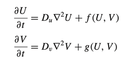
Alan Turing suggested that pattern formation in animals is a result of a break in homogeneity (Turing, 1952). He proposed that through the diffusion and reaction of chemical morphogens, patterns can arise (Woolley et al., 2017). These reactions are based on the presence of activators and inhibitors who have conflicting operators. Activating agents self-multiply, while inhibitors enforce regulation through negative feedback (Woolley et al., 2017). When a disturbance is introduced into this mixture, a variety of patterns can be created, and this mechanism will be explained in further detail (Turing, 1952).
Like many mathematical models, initial conditions are required. The first requirement is that the inhibitors and activators must exist in a stable state (Woolley et al., 2017). The second condition is that this equilibrium must be disturbed once diffusion is introduced (Woolley et al., 2017). Although diffusion is normally interpreted as a stabilising agent, homogeneity can be lost when multiple components are displaced at the same time. In short, Turing proposed a diffusion-driven instability model as a mechanism for pattern formation (Kimura, 2014). The following section will discuss how diffusion can be used to create patterns and what parameters allow for animal uniqueness.
Chemical Pre-Patterns
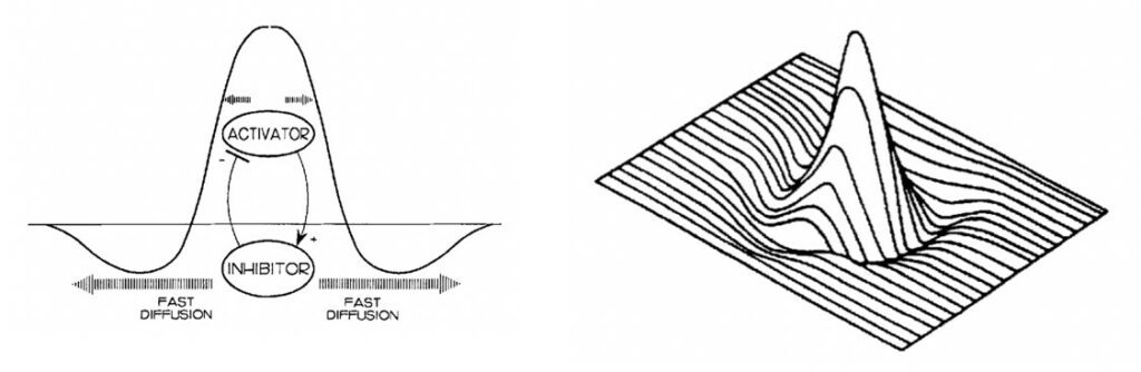
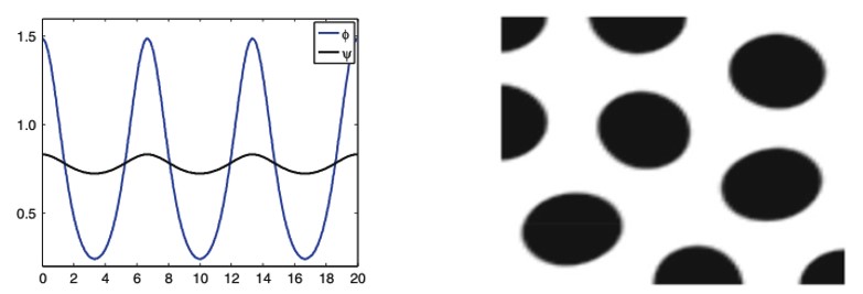
As previously mentioned, patterns form through the interaction of inhibitor and activator chemicals and without diffusion, no patterns can be produced (Woolley et al., 2017). The autocatalytic nature of the activators is suppressed by the rapid diffusion of inhibitors (Oster & Murray, 1989). This results in regions with high concentration of activator molecules, surrounded by zones of inhibition (Oster & Murray, 1989). The following landscape then serves as the chemical pre-pattern for the organism's cells to react to. With the chemical pre-pattern set, morphological traits, like patterns, can then be filled in as the organism's cells begin reading the instructions (Oster & Murray, 1989). Importantly, colourations only form in the regions of local activation. Zones of inhibition essentially provide the breaks in patterns, which can be seen clearly in Figures 2 and 3.
Spatial Dependence
In the living ecosystem, there are many examples of animal patterns. Whether it be simple spots as shown in Figure 3 or stripes, no two animals express the same pattern (Oster & Murray, 1989). Such differences are a result of variances within their respective chemical pre-patterns (Oster & Murray, 1989). Each animal has a unique set of starting conditions, which impacts the final distribution of inhibitors and activators (Oster & Murray, 1989). This is of no surprise as with any mathematical expression, one can drastically alter the product mapped by a function by adjusting the variables in question.
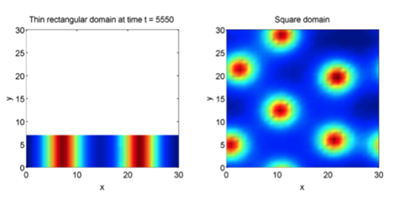
A key parameter that is worth discussing is the effect of domain size on pattern appearance (Kimura, 2014). As explained earlier, chemical reactions occurring between inhibitors and activators take place over a specific region of space. Within this region, these chemicals shift from a well-mixed homogeneous state to a more disruptive distribution as seen in Figure 2. With this being said, these activators and inhibitors need space in order to rearrange themselves (Kimura, 2014). If the domain is too restricted, the chemicals remain in equilibrium, hence no pattern. When the domain size increases, the overall complexity and degree of heterogeneity is significantly improved as shown in Figure 4, 5 and 6 (Woolley et al., 2017).

To summarise, the above discussion presented a simple description of Alan Turing's reaction-diffusion model. His mathematical approach allowed for the understanding of pattern formation in nature, a concept that was seemingly impossible to uncover through biological investigation alone. Through a theoretical system of chemical reactions and diffusion, Turing was able to provide a mathematical model for the existence and formation of patterns in animals. Although the natural world does not always agree with his modeling, Turing set the groundwork for further experimentation in this field.
Disruptive Colouration
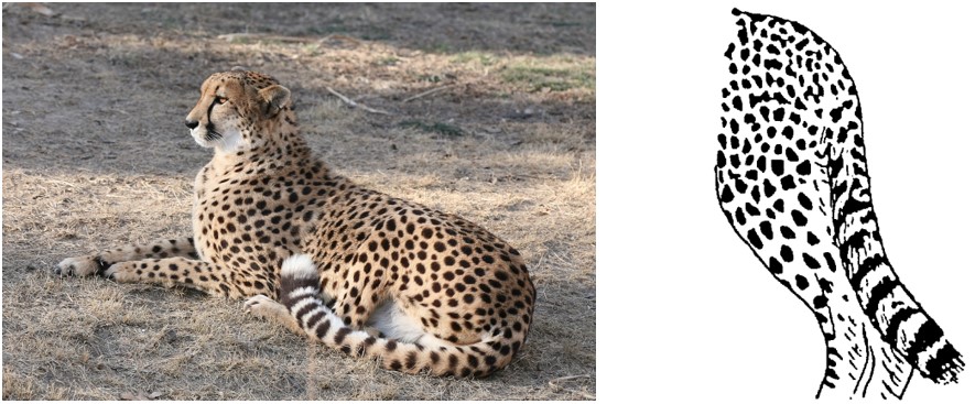
Although pattern matching is an effective way for animals to camouflage and hide from their predators, any differences between the animals' pattern and its background, such as a shadow or body outline, might reveal their location. To overcome this issue, some animals have adapted to using opposing shapes and patterns on their body to break up their form (Espinosa & Cuthill, 2014). This is known as disruptive colouration is a type of camouflage where animal's contrasting markings break up their overall body outline and create false edges (Troscianko et al., 2017). An example of this is seen in the cheetah (Figure 7), whose markings can not only help hide them in the grass from predators, but also acts as an aid in hunting.
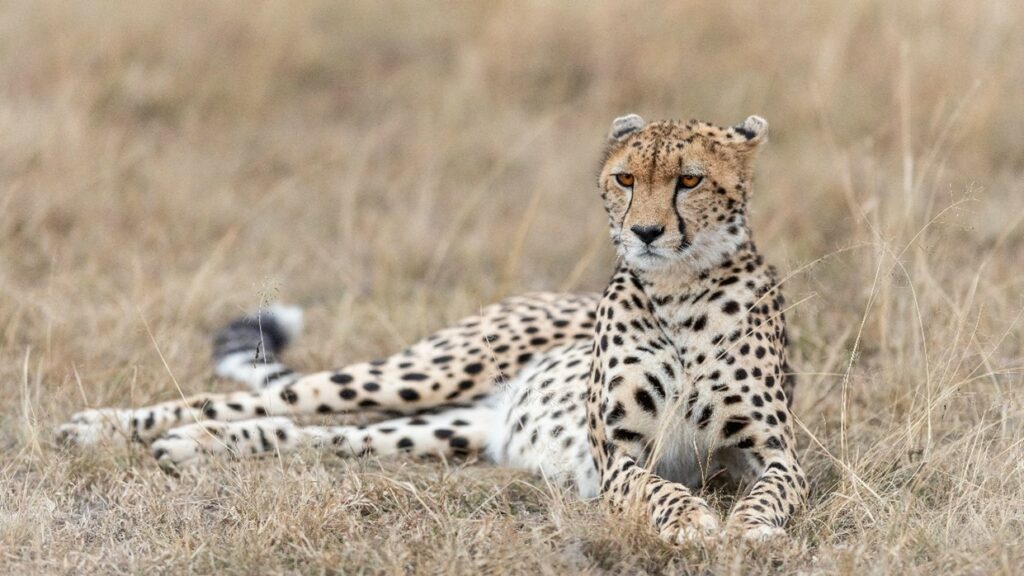
This theory of disruptive colouration was proposed by Thayer in 1909, and suggests that strong contrasting geometric shapes and patterns can break up an animal's form, and ultimately give viewers the impression of a series of distinct and seemingly unrelated objects (Espinosa & Cuthill, 2014). This provides an advantage for target animals since even though their predators may see elements of the disruptively coloured animal, the high-contrasting markings crossing the animal's outline disrupt the viewer's ability to detect it separately from its background (Troscianko et al., 2017).
Saliency Mapping
Saliency is a way to quantitatively determine how distinct an animal's markings are from their surrounding visual environment (Pike, 2018). An animal with high salience has a large contrast to its background and can very easily be detected, whereas low salience is the opposite. Thus, camouflaging animals using disruptive colouration aim to minimize their salience to their surrounding background. Since salience is merely an interaction between the animal's appearance and its environment, an animal well camouflaged to one background may have high salience against another (Pike, 2018). Therefore, quantifying salience must consider the relative characteristics of both the target and the background, and this is achieved in a technique called saliency mapping.
Saliency maps are computational topographic models of a scene that describes how likely human gaze will be fixed to a certain location (Skurowski & Kasprowski, 2018). It is a model of “bottom-up” visual attention, which reflexively directs visual focus based on certain low-level visual features like colour, orientation, and/or brightness contrasts (Pike, 2018). The overall schematic of a salience map is seen in Figure 8, below.
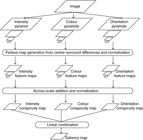
Construction of a Salience Map
To construct a salience map, RGB images are inputted and for each, a Gaussian pyramid is constructed by repeatedly low-pass filtering and subsampling the image to produce a sequence of reduced-resolution images (Pike, 2018). Each level of this pyramid is then further broken down into a series of “maps” that correspond to the visual features of intensity, colour and orientation. From here, a series of feature maps are created which encode local intensity, colour and orientation contrasts (Pike, 2018). These feature maps are then combined hierarchically first into three conspicuity maps for intensity CI, colour CC, and orientation CO. These conspicuity maps are then linearly combined to form a single overall saliency map S, using the weighting factors wf of each conspicuity map that contribute differentially to saliency (Pike, 2018). Overall, the resulting saliency map can be denoted by:
S = wICI + wCCC + wOCO
In a constructed salient map, darkly coloured parts represent low salient regions and lighter colours signify regions of high salience, as seen in Figure 9 below. This figure demonstrates the conspicuity maps for colour, luminance and orientation (b-d) of a displaying peacock, and its overall salience map in (e).
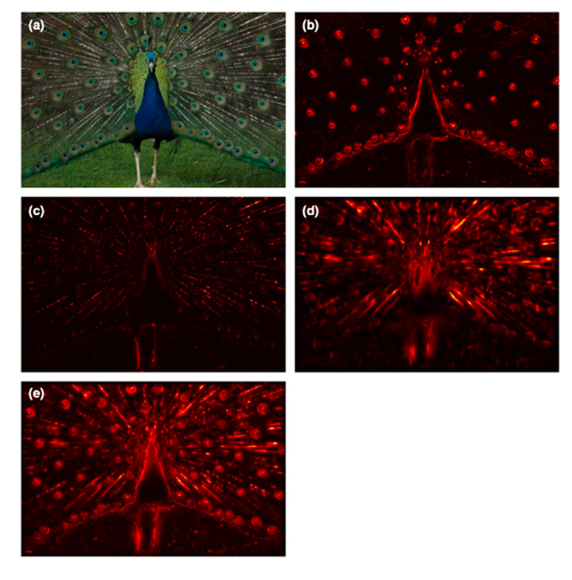
From these maps, one can see that the light red regions indicate the low salience regions of the peacock, the parts that are best camouflaged to its background. From the overall salience map, it is evident that these low salience regions are mostly found at the peacock's body outline, which align with the principles of disruptive colouration. The most salient, or distinct, parts of the peacock, as shown in the dark red-black regions, are scattered throughout the peacock's body, giving it a divided body outline and false edges. This demonstrates the effects of disruptive colouration for the peacock because it allows us to see which parts of the peacock are first noticeable by predators. The majority of the peacock has a low salience meaning that it is well blended into its visual environment and gives predators a hard time detecting it from far away.
Optimization of Countershading Techniques
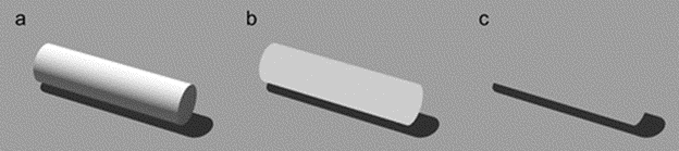
Although environments vary greatly and the perception of angle of predators to prey differ, the goal of countershading is to be perceived as a uniform object which blends in with the rest of the environment. Having a dark pigment on the upper surfaces of the body and a light pigment on the underside creates a counterillumination effect where the shadow is negligible and the three-dimensional shape of the animal seems flat, thus blending in with its surroundings (Cuthill et al., 2016). Although the concept seems simple, the goal will be to optimize different radiance, iridescence, and reflectance combinations to describe the best countershading possible for animals.
The two main categories of countershading are background matching (BM), which focuses on the reflectance and iridescence of the body compared to its background, and obliterative shading (OS), which aims to create the two-dimensional effect through radiance gradient, shading, and colouration (Penacchico et al., 2015). In optimal cases, the OS also has BM qualities, and is considered perfect obliterative shading (OS+) (Figure 10).
The modeling for countershading will be broken down into the BM, OS, and OS+ section since each of these types have different limitations and characteristics. For BM the goal is to have little to no difference with the environment; the product of the body's iridescence and reflectance should match the radiance of the background (Penacchico et al., 2015). Moreover, supposing that the animal's reflectance is Lambertian, it can be chosen by the inverse of its iridescence pattern, conditional to the maximal reflection being less than or equal to 1 (Penacchino et al., 2017) (Equation 1). While the possibility of achieving homogenous BM is unlikely (reflectance difference of 0), due to the areas of the body which receive minimal amounts of light, the areas of the body which are highly exposed can match the darker shades of their environment by having a low reflection.
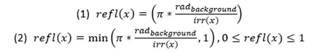
Since the goal of OS is to deceive the perception and create a seemingly two-dimensional colouration, the gradient and the reflectance of the animal's skin must match the environment colour as well as create a gradient to hide its shadow (Cuthill et al., 2016). Although colour throughout the body will differ, the goal is to model based on the iridescence and reflectance of the animal's integument. Unlike BM, an animal's skin can have a gradient pattern which matches the requirement, therefore, giving light to the OS+ formula (Pennacchico et al., 2015) (Equation 2).
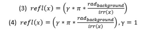
Equations 1 and 2 are pertinent in general terms, more specifically, when the reflection of the light is uniform and specular. Moreover, they do not contain a factor for the colour of the light. The modification of the equations simply required the input of the wavelength felt on the location, thus making the equation a two variable function (Penacchico et al., 2015) (Equation 3).
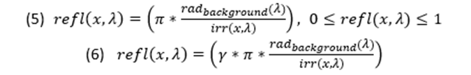
Although the equations are accurate as generalized solutions in simple settings, they may be complicated when ambient lighting is more complex (varying temperature or time of day), within a different medium (like water), or from different angles of perception (Cuthill et al., 2016). The models presented are for simple cases and present possible calculations using quantitative values of the reflectiveness and iridescence of the animal's surface, thus concrete live examples of these concepts have not yet been evaluated. Yet by intuition it is clear that the counter shadowing required for a small surface fish with high iridescence and blue colours would be extremely different from the calculations required for a large deep-water fish due to the characteristics of light in water as well as the shape and or the animal.
Motion Camouflage
When in movement, camouflaging traits are not always effective because they “produce a contrasting image against a stationary background” (Pembury Smith & Ruxton, 2020). To help counter this effect, some species of animals have developed behaviours to remain camouflaged whilst they are moving around. This is called motion camouflage.
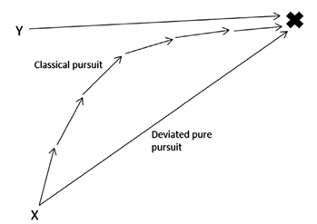
Motion camouflage, also known as optic flow mimicry, describes the “motion of elements relative to an observer moving through an environment” (Troscianko et al., 2009). In other words, this type of camouflage plays with the point of view of an individual that is travelling in a certain direction. Motion camouflage is mostly used by individuals that are trying to catch their prey without being noticed. They realized that if they follow a specific path, they can remain in a fixed position in the eyes of their prey. This motion can be explained by mathematical equations and sketches (Figure 14). The alternative to this type of pursuit is called classical pursuit. This is when the predator just tries to catch up to its prey by following its path (Pembury Smith & Ruxton, 2020). However, this mode of pursuit is only successful if the predator has the capability of at least matching the speed of the prey. So slower predators will have a lot of trouble getting the resources they need especially if the preys follow an unpredictable path when escaping.
The reason why this method works is based on three principles. The predator needs to be aware of the motion and the distance it has from the prey and the distance it has from a fixed stationary point (Troscianko et al., 2009). This fixed point is key because it is what the prey bases itself on to believe that the moving predator is still. The predator must remain on the line connecting the prey and the fixed point for this illusion to work, this line is called the camouflage constraint line (Pembury Smith & Ruxton, 2020). As it stays on this line it gradually decreases the distance between it and the prey it is trying to catch to eventually be close enough to attack. This is what is called the principle of constant bearing and decreasing range (Pembury Smith & Ruxton, 2020). The only possibility of detection in this case would be from the increase in size of the predator as it approaches (Pembury Smith & Ruxton, 2020) but this is not as detectable as if the predator left the line it's supposed to stay on.
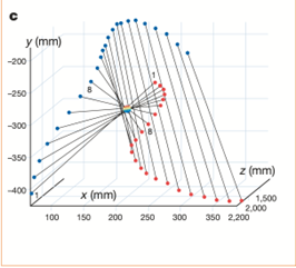
There are two types of reference points a predator can base itself upon. One of them was the previously talked about case where the fixed point is known and usually this point is the initial position of the predator (Troscianko et al., 2009). The other case is where the fixed point lies at infinity (Troscianko et al., 2009). This type of fixed point is when the background the predator is trying to look fixed in is very far away as opposed to a landmark like a rock in the first case. The second type is mostly used in aerial situations (Figure 15).
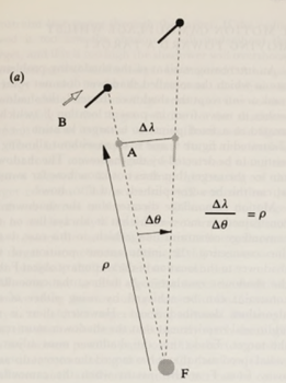
There is an equation that relates a predator's position to the principle of motion camouflage. The ratio between the changes in lateral distance and angle must equal the distance the predator makes with the fixed point must be kept constant. This mathematical relationship is shown in Figure 16.
A more sophisticated equation can be constructed to model more complex trajectories that don't necessarily follow straight lines given as follows:
r(t) = r(0) + u(t)(z(t) – r0)
Here, z(t) represents the position of the prey and r(t) represents the position of the aggressor. Also, r0 represents the fixed point of reference (Glendinning, 2004). This equation allows the prediction of the path the predator will follow with the known path the prey will follow with the assumption that the velocity is kept constant (Glendinning, 2004).
In the cases where there are many preys in different locations, it makes the job of the predator much harder because there are not always obvious locations to be seen as fixed in the eyes of multiple individuals. There is, however, a location to “minimize the shadowers motion” (Srinivasan & Davey, 1995). Overall, though, when there are more individuals, this concept does not apply too well. In general, the mathematical model for motion camouflage was created with the goal of explaining the behaviour of predators hunting habits and may oversimplify certain aspects in order to understand them more clearly.
Conclusion
Overall, mathematics and computational programming plays an important role in describing and understanding camouflaging techniques in animals. Turing's reaction-diffusion model aims to explain different pattern formations in animals. Saliency mapping provides a method to visualize the way disruptive colouration provides false definitions of an animal's outline to make them harder for predators to detect. Similarly, maximizing countershading through a combination of different radiance, iridescence and reflectance provides an optimal way for an animal to blend in with its surroundings. As well, the direction and mechanisms of motion camouflage can be interpreted and analyzed by various graphing and modelling techniques.
References
Barrio, R. (1999). A Two-dimensional Numerical Study of Spatial Pattern Formation in Interacting Turing Systems. Bulletin of Mathematical Biology, 61(3), 483-505. https://doi.org/10.1006/bulm.1998.0093
Cheetahs. (n.d.). Rare Gallery. Retrieved December 12, 2021, from https://rare-gallery.com/874738-cheetahs-grass-lying-down.html
Cuthill, I. C., Sanghera, N. S., Penacchio, O., Lovell, P. G., Ruxton, G. D., & Harris, J. M. (2016). Optimizing countershading camouflage. Proceedings of the National Academy of Sciences, 113(46), 13093-13097. https://doi.org/10.1073/pnas.1611589113
Espinosa, I., & Cuthill, I. C. (2014). Disruptive Colouration and Perceptual Grouping. PLOS ONE, 9(1), e87153. https://doi.org/10.1371/journal.pone.0087153
Glendinning, P. (2004). The mathematics of motion camouflage. Proceedings of the Royal Society of London. Series B: Biological Sciences, 271(1538), 477-481. https://doi.org/doi:10.1098/rspb.2003.2622
Herrero, M. A. (2007). On the role of mathematics in biology. Journal of Mathematical Biology, 54(6), 887.
Kimura, Y. T. (2014). The Mathematics of Patterns: The modeling and analysis of reaction-diffusion equations [Thesis, Princeton Univeristy]. https://www.pacm.princeton.edu/.
Mizutani, A., Chahl, J. S., & Srinivasan, M. V. (2003). Motion camouflage in dragonflies. Nature, 423(6940), 604-604. https://doi.org/10.1038/423604a
Oster, G. F., & Murray, J. D. (1989). Pattern formation models and developmental constraints. Journal of Experimental Zoology, 251(2), 186-202. https://doi.org/https://doi.org/10.1002/jez.1402510207
Pembury Smith, M. Q. R., & Ruxton, G. D. (2020). Camouflage in predators. Biological Reviews, 95(5), 1325-1340. https://doi.org/10.1111/brv.12612
Penacchio, O., Harris, J. M., & Lovell, P. G. (2017). Establishing the behavioural limits for countershaded camouflage. Scientific Reports, 7(1). https://doi.org/10.1038/s41598-017-13914-y
Penacchio, O., Lovell, P. G., Cuthill, I. C., Ruxton, G. D., & Harris, J. M. (2015). Three-Dimensional Camouflage: Exploiting Photons to Conceal Form. The American Naturalist, 186(4), 553-563. https://doi.org/10.1086/682570
Pike, T. W. (2018). Quantifying camouflage and conspicuousness using visual salience. Methods in Ecology and Evolution, 9(8), 1883-1895. https://doi.org/https://doi.org/10.1111/2041-210X.13019
Skurowski, P., & Kasprowski, P. (2018, 12-14 Dec. 2018). Evaluation of Saliency Maps in a Hard Case – Images of Camouflaged Animals. 2018 IEEE International Conference on Image Processing, Applications and Systems (IPAS),
Srinivasan, M. V., & Davey, M. (1995). Strategies for active camouflage of motion. Proceedings of the Royal Society of London. Series B: Biological Sciences, 259(1354), 19-25. https://doi.org/doi:10.1098/rspb.1995.0004
Troscianko, J., Skelhorn, J., & Stevens, M. (2017). Quantifying camouflage: how to predict detectability from appearance. BMC Evolutionary Biology, 17(1), 7. https://doi.org/10.1186/s12862-016-0854-2
Troscianko, T., Benton, C. P., Lovell, P. G., Tolhurst, D. J., & Pizlo, Z. (2009). Camouflage and visual perception. Philosophical Transactions of the Royal Society B: Biological Sciences, 364(1516), 449-461. https://doi.org/doi:10.1098/rstb.2008.0218
Turing, A. M. (1952). The Chemical Basis of Morphogenesis. Philosophical transactions of the Royal Society of London. Series B, Biological sciences, 237(641), 37-72. http://www.jstor.org/stable/92463
Woolley, T. E., Baker, R. E., & Maini, P. K. (2017). Turing's Theory of Morphogenesis: Where We Started, Where We Are and Where We Want to Go. In (pp. 219-235). Springer International Publishing. https://doi.org/10.1007/978-3-319-43669-2_13