Mathematical Modeling of the Antler Growth Cycle

Laurianne Daoust, Félix Lavoie, Annabelle Huynh-Rondeau, Erica Song

Abstract

Antler regeneration is a complex process unique in nature because of its year-long perpetual cycle. Although antlerogenesis is a process shared by all males in the Cervid family, many factors affect individual antler growth and the characteristics of individual antlers. This paper will discuss these factors and their effect on antlers through mathematical models and equations. Particularly, the inversely proportional relationship between antler size and the annual survival rate among deers will be explained through the Handicap Principle. Furthermore, the linear relationship between antler velvet yield and pre-rut live weight of deers will be analyzed in three different age groups. An analysis of the exponential connection between age and the percentage of maximal antler size will also be provided. Additionally, trophic memory, the effect of antler injuries on future antler cycles, will be discussed through linear encoding. Finally, the paper will touch on photogrammetry, an imaging technology that exploits mathematic principles to extract information from photographs of antlers.

Introduction

An organism's evolutionary fitness is measured by its ability to mate and pass on genetic material to offspring. Species spanning the Kingdom Animalia have evolved marvelous ornaments to attract mates, which does not come without a cost. In the context of Cervidae, or the family of ruminant mammals, the presence of antlers allows males to gain high social ranking and access to mates through physical combat. These spiky structures are anchored in the individual's skull and follow a yearly regenerative cycle—the antler growth cycle. However, antlers are hypothesized to follow the handicap theory, which suggests that the bigger and more intimidating antlers—although recognized by females as an indicator of possessing the best genes to mate—hinders their longevity of survival in the wild. Thus, mathematical models can be utilized to better understand the survival rate of antlers as a function of reproductive success.

Similarly, the antler growth cycle follows a yearly interval, growing from bony pedicles in early spring and cast in the last weeks of March. The growth rate is affected by various factors, namely nutrition, genetics, and age, which can be modeled mathematically to spark insight on the trend followed by the antlers' growth rate under each factor. This rate varies among various species of the Cervidae family, namely, elk, red deer, and white-tailed deer. 

This essay will demonstrate how mathematical models can be used to illustrate the relationships between antler size, reproductive success, and survival rate. Likewise, the relationship between the antler growth rate, size, and velvet weight and various factors such as genetics and age will be discussed. Moreover, the linear relationship between casting time, nutrition, pre-rut bodyweight and antlers will be elucidated. Finally, we will address the innovative potential of antlers in biomimetics, where parametric 3D Computer-Aided Designs are utilized to create antler 3D models, and in regenerative medicine, where a linear-encoding model is used to study antler morphology.

The handicap principle: advantages and disadvantages of deer antlers

Darwin suggested that both natural and sexual selection are responsible for the evolution of mating ornaments (Clifton et al., 2016). While natural selection is the process through which an organism adapts to its environment, causing alterations in the heritable traits of a population over generations, sexual selection leads to shifts in traits based on an individual's ability to reproduce. Zahavi's handicap theory suggests that the bigger and most beautiful ornaments—for instance, the largest and most imposing antlers—are damaging to their bearer's health. However, ornaments are symbols of genetic quality, as they prove that their carriers can survive the challenge of carrying such heavy architectures, and thus females will prefer to mate with males carrying larger antlers (Clifton et al., 2016; Clutton-Brock, 2007; Nur & Hasson, 1984). Moreover, evidence has shown that antler size is directly proportional to fighting ability, so males with stronger antlers are more likely to mate and pass on genetic material (Clutton-Brock, 2007; Nur & Hasson, 1984). 

The antler growth cycle is a yearly considerable investment. The growth of antlers feeds on the deer's calcium reserves, allowing the antlers to weigh up to 20 kg or more. Besides draining calcium storage, large and bulky antlers prevent deer from swiftly escaping predators, thus posing a threat to their survival. Therefore, as illustrated in Figure 1, the antler size (length and width) (x) is inversely proportional to the annual survival rate of deer. 

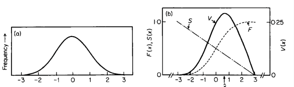
Fig. 1 Multiplicative model. (a) Frequency distribution of the male deer handicapping trait, with x corresponding to the standardized value of the trait. (b) Relationship between antler size, mating success (F) and survival rate (S). V (=F·S) is proportional to the overall fitness (Nur & Hasson, 1984).

Since the male mating success (F) depends on competition with other males, F is proportional to the male's social ranking in the population. The expected annual reproductive output of an organism in the population is related to the product of F(x) and S(x), termed V(x) (Nur & Hasson, 1984). Knowing that S corresponds to the probability of a male Cervidae to survive from the previous mating season to the time of breeding and that the male's expected fecundity equals F·a (where a corresponds to the expected number of offspring produced), the male's animal reproductive output is equivalent to S·F·a. Thus, expected yearly reproductive output demonstrates a clear correlation to a Darwinian fitness model in which the population is stationary, as is likely for populations of large mammals (Nur & Hasson, 1984; Schaffer, 1983). 

As portrayed in Figure 1, for different values of F and S, V(x) peaks at an intermediate value of x, corresponding to the optimum antler size. Now, let's consider the individual reproductive potential (ind) in relation to the antler size. Since antlers have both ornamental and practical values (e.g., in rare cases, the antlers can serve to defend against predators) but are harmful beyond a certain size, there exists an optimal antler size which can be expressed with the following formula, assuming a quadratic form (Clifton et al., 2016):

\begin{equation}
\phi^{(ind)}=a(2a_{opt}-a)
\end{equation}

Here, a_opt corresponds to the optimal ornament size, and a to the ornament size. According to Zahavi's handicap principle, we expect healthier organisms to be able to support heavier and larger ornaments. In other words, we expect the optimal ornament size, a_opt, to increase proportionally to intrinsic health, h (Clifton et al., 2016):

\begin{equation}
a_{opt}=a_{opt}\cdot h
\end{equation}

Figure 2 illustrates the general shape for the individual reproductive potential function.

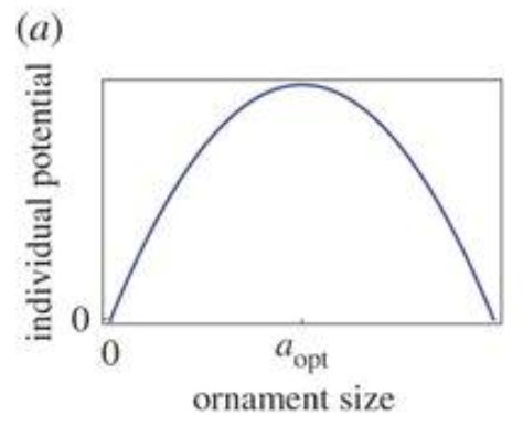
Fig. 2  Example of individual potential quadratic function. Ornament size increases with respect to the individual potential until the optimal ornament size is reached, after which the curve descends. (Adapted from Clifton et al., 2016).

Consider now the sexual reproductive potential, φ^(soc), which represents the drive for competition between males to mate with females. Social potential is proportional to ornament size, as larger and stiffer antlers allow males of higher social rank to win battles and access females, and the latter prefer males with more extravagant antlers (Clifton et al., 2016; Nur & Hasson, 1984). Here, the social potential is chosen to be a power of the difference between antler size and the Cervidae population's average antler size. For monotonicity, the social reproductive potential is antisymmetric to the average antler size, thus resulting in a formula for the social potential (Clifton et al., 2016):

\begin{equation}
\phi ^{(ind)}= sgn(a-\bar a)\rvert a-\bar a\lvert^\gamma
\end{equation}

Here, sgn is the sign function, an odd mathematical function which extracts the sign of a real number, γ represents the rate of deviation from the mean influence reproductive potential, and a is the average antler size in the Cervidae population. The parameter γ mainly refers to female choice, as females tend to favor male deer with larger antlers. This parameter is considered constant, as female choice evolves on a slower time scale than male ornamentation (Lande, 1981; Clifton et al., 2016). Figure 3 shows an example of the social reproductive potential function.

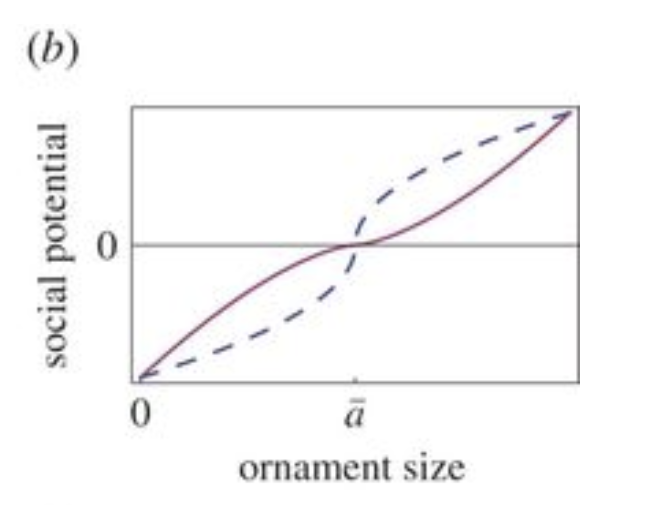
Fig. 3 Example of social potential quadratic function, antisymmetric about the population mean, ā. Here, different values of γ were chosen: blue dashed is γ = 0.5, and maroon solid is γ = 1.5 (Adapted from Clifton et al., 2016).

As both natural and sexual selection lead to the evolution of mating ornaments, we consider the total reproductive potential as the weighted average (Clifton et al., 2016):

\begin{equation}
\phi=S\phi ^{(soc)}+(1-S)\phi^{(ind)}
\end{equation}

Here, S tunes the importance of competition between organisms in the population (e.g., sexual selection) in comparison to individual drive for survival (e.g., natural selection) (Clifton et al., 2016). Figure 4 illustrates examples of total potential functions.

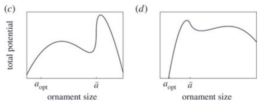
Fig. 4 Examples of total reproductive potential function. (c) Here, γ < 1. Two local maxima can be observed, corresponding to two distinct morphs. The largest ornament morph has the highest potential (here, γ= 0.5). (d) Here, 1 < γ < 2. Two local maxima are observed, corresponding to two distinct morphs. The smallest ornament morph has the highest potential (γ= 1.5) (Adapted from Clifton et al., 2016).

If we assume that evolutionary forces optimize the reproductive potential at a rate which is proportional to the advantages of displaying ornaments, such as antlers, the ornament size can be expressed using the following dynamics (Clifton et al., 2016):

\begin{equation}
\frac{\partial a}{\partial t}=c\frac{\partial \phi}{\partial a}
\end{equation}

Here, the time-scaling parameter, c, is superior to 0. The phenotype flux, da/dt represents how the distribution of various ornament sizes in a large population of Cervidae changes over large scales of time due to natural or sexual selection. Finally, putting all these equations together, we obtain a piecewise-smooth ordinary differential equation that represents the antler size flux in a population of Cervidae of size N (Clifton et al., 2016): 

\begin{equation}
\frac{da}{dt}=c\left[s\gamma(1-\frac{1}{N})\lvert a-\bar a\rvert ^{\gamma-1}+2(1-s)(a_{opt}-a \right]
\end{equation}

Therefore, by plugging in values for all variables except for the optimal ornament size, one can find the ideal antler size in a population of red deer, for instance. Thus, these perfectly suitable dimensions will simultaneously allow males to attract females for mating and win dominance battles, without significantly hindering their survival in nature.

Factors affecting antler growth and size, casting date and weight of antler velvet

Antler growth, antler size, casting date and weight of antler velvet do not remain constant between individuals. Instead, they depend on multiple factors, including bodyweight, nutrition, genetics, and the age of the individual.

The effect of nutrition and bodyweight on antler casting date and antler velvet yield

A study was constructed by the Animal Science Department of Lincoln College in New Zealand to determine whether better winter nutrition results in an early casting date and a higher yield of velvet. The experiment observed the effects of nutrition on two different Cervids farms: Farm H and Farm L. Each farm was subdivided into three groups, each given a different amount of pasture, hay, and pellets. The average food intake in kilograms per day for each group is tabulated in Table 1 (Muir & Sykes, 1988).

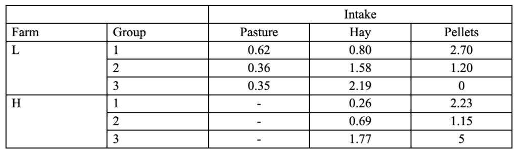
Table 1 Average individual intake of pellets, pasture, and hay of different herds of red deer during winter (Muir & Sykes, 1988).

In farm H, no pasture was given to the deer. Overall, more food was given to the red deer herds in farm L than to the herds in farm H.  Differences in average bodyweight and antler casting dates were observed in these conditions. The differences in mean bodyweight values and casting dates are given in Table 2 (Muir & Sykes, 1988).

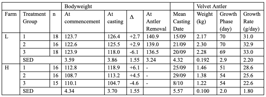
Table 2 Bodyweight, Mean Casting Date and Velvet Growth Rate of Velvet Antler of Different Herds of Red Deer during Winter (Muir & Sykes, 1988).

The results obtained in Table 2 are related to the different nutrition of each group of deer. The growth rate of antler velvet in Farm L, where animals were given much more food than Farm H, is significantly higher. The length of the growth phase is also higher in farm L than in farm H.  Furthermore, Table 2 suggests that a delayed casting date corresponds to a smaller velvet weight.  

Statistical analysis was done on the results, which concluded that there is a relationship between antler casting date and bodyweight. This relationship depends on the antler cycle stage in which the weight of the individual is measured. In these equations, Y represents the date of antler casting while X represents the body weight in kilograms. If the weight is measured in winter, equation (7) will represent the date of antler casting.

\begin{equation}
Y=132.2-0.338X
\end{equation}

If the weight is measured at the time of antler casting, equation (8) will represent the date of antler casting.

\begin{equation}
Y=113.2-0.184X
\end{equation}

If the weight is measured at the time of velvet removal, equation (9) will represent the date of antler casting.

\begin{equation}
Y=126.1-0.257X
\end{equation}

Finally, if the weight is measure right before the rut, equation (10) will represent the date of antler casting.

\begin{equation}
Y=146.5-0.344X
\end{equation}

In all these cases, the date of antler casting is linearly related to their weight. Poorly nourished individuals experience delayed antler casting dates. In fact, poor nutrition is associated with a delayed decline in testosterone in the bloodstream. Since testosterone prevents antler casting, this deferred decrease in testosterone levels explains the relationship between nutrition and antler casting date (Muir & Sykes, 1988).

As shown in Figure 5, the rate of antler growth differs between the two farms. Results show that the average weight of antler velvet is 1.36 ± 0.045 kilograms in farm H, while the average weight of antler velvet in farm L is 2.25±0.076 kilograms. Due to the significant difference between the average weight of antler velvet produced by each farm, the study concluded that good winter nutrition is associated with a higher antler velvet yield (Muir & Sykes, 1988). 

A linear relationship was also observed between bodyweight and velvet yield. This relationship was studied in three age groups: 3, 4, and 5 years old. Figure 5 illustrates this relationship for each age group. The bottom line is associated with the group of 3 year olds, the middle line with the 4 year olds, and the top line with the 5 year olds.

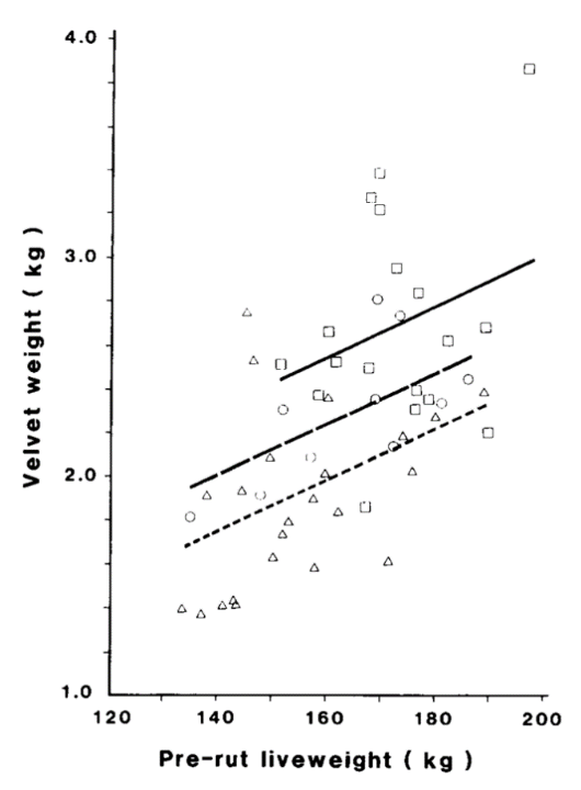
Fig. 5 Linear Relationship between Pre-rut Liveweight and Velvet Weight of Groups of 3 (D), 4(o), and 5(□) Year Old Stags of farm L (Muir & Sykes, 1988).

Figure 5 illustrates that the velvet weight is directly proportional to the pre-rut liveweight of the deer. The slopes of all three functions of velvet weight are identical: for each increase of 10 kilograms in liveweight, an increase of 0.12 kilograms of velvet weight was observed for all age groups. However, velvet weight is demonstrated to increase with age due to the increase in pedicle diameter (Muir & Sykes, 1988). 

Overall, this study suggests bodyweight has a greater impact on antler weight than nutrition. However, poor body conditions, namely malnutrition, delay the date of antler casting, which in turn is related to a lower antler velvet weight.

The heritability of antler characteristics

The Texas Parks and Wildlife Department studied the influence of genetics on antler characteristics. To do so, nine genetic lines of deer were put under observation. However, two significantly different lines were observed in more detail due to the considerable difference between their two sires. The first genetic line, called the “fork,” came from a sire with 6.5 antler points at 18 months (Harmel et al., 1988). The number of points of a buck is the number of tines on its antlers. It is also associated with the quality of its nutrition and its genetics (McMahon, 2022). The second line, called “spike,” came from a sire with 2.5 antler points. Every year, measurements of the number of points (TP), the bodyweight (WT), the circumference of antler base (BC), the length of the main beams (MB), the weight of antlers (AW) and the maximum inside spread of the beams (SP) were recorded for each buck in the genetic line (Harmel et al., 1988). The measurements recorded at 1.5, 2.5, and 3.5 years of age for the fork and spike lines are tabulated in Table 3.

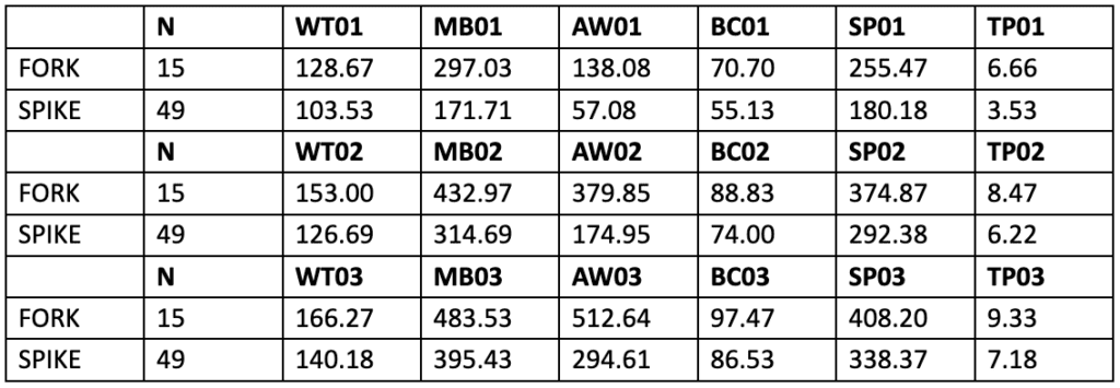
Table 3 Average Antler Characteristics of the Fork Line and the Spike Line at 1.5, 2.5, and 3.5 Years of Age (Harmel et al., 1988).

This table shows that the genetic line of the sire with the greatest number of antler points has better antler characteristics than the genetic line of the sire with the lowest number of antler points. Since for all age groups, the average of every antler characteristic observed was greater for the Fork line than the spike line; the study concluded that antler traits are heritable (Harmel et al., 1988).

The relationship between age and antler growth

Antler growth is also related to the age of the Cervid. During their 5 first months, bucks only grow button bucks. Between 12 and 18 months, a buck grows its first antlers. Antler size continues to increase until the maximum size is attained, around 6.5 years of age. The percentage of maximal growth as a function of age is shown in Figure 6 (Pierce et al., 2022).

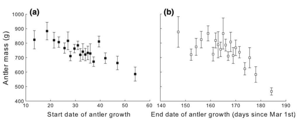
Fig. 6 Antler Mass as a Function of Start (a) and End (b) Dates of Antler Growth (Clements et al., 2010)

The figure above shows that the later the antler growth phase, the lighter the antlers are. Following this principle, it is possible to approximate antler mass if the start and end dates of the growth phase are known. For instance, Figure 7 relates antler size to the start and end dates of antler growth through a linear model for an 8 year-old male red deer living in average environmental conditions.

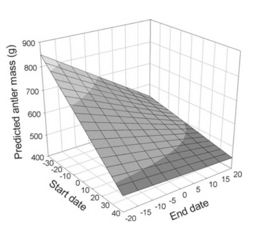
Fig. 7 Linear model of the predicted antler mass of an 8-year-old red deer as a function of start and end date of the antler growth phase (Clements et al., 2010). The observed plane illustrates that the earlier the start date of antler growth, the heavier the antlers will be.

Variable target morphology in antler regeneration

For comparison, the amputation of a salamander leg clearly demonstrates a remarkable regenerative process that restores the original morphology after only one month of growth back to its former size. (Iten and Bryant, 1973). In most species with regenerative capacity, such as salamanders, the regenerative process produces the same desired morphology. However, in some regenerating species like deer, physical interventions or injuries can directly modify the target morphology that their regenerative process restores.

Antlers are yearly shed and rebuilt deer appendages that grow from bone tissues called pedicles. In general, only male deer develop antlers through a cyclic process aligned with the natural light cycle. As seen in Figure 8, regenerating antlers have a dense vascular network and many sensory fibers that sprout from the pedicle. When growth ceases, bone is generated, and the velvet dries and sheds, leaving only the exposed solid bone (Goss, 1983). Finally, the antlers are shed after the mating season, and a new cycle begins.

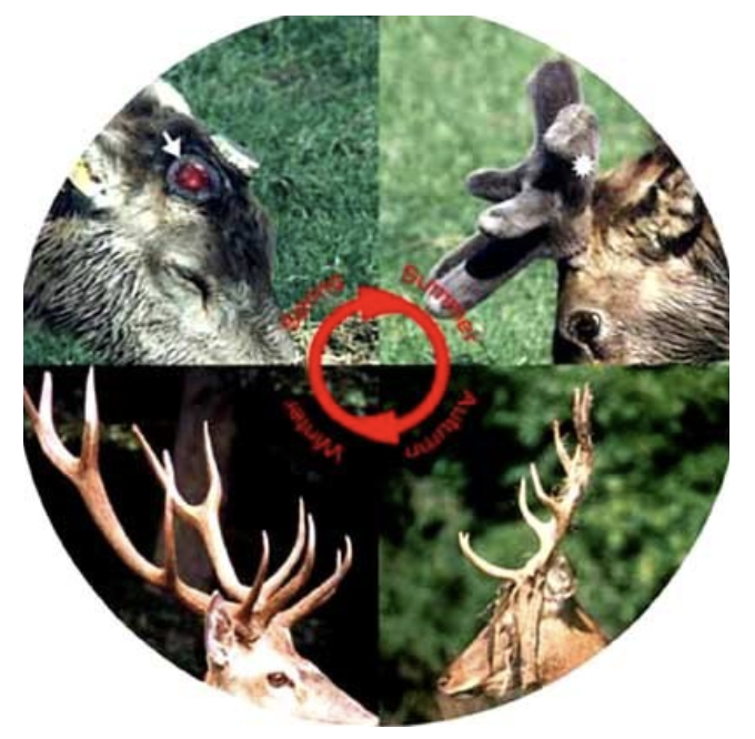
Fig. 8 Hard antlers fall off the pedicles (arrow) in the spring, and antler regeneration occurs promptly. Summer is a time of rapid antler growth. Velvet skin surrounds developing antlers. Antlers become fully calcified in fall, and velvet skin begins to slough. Hard antlers are connected to their pedicles in the winter and cast the following spring, triggering a new round of antler regeneration (Li et al., 2009).

During the early years of life, there is no huge difference in the antler's shape. Until maturation, the number of branches and length increases with age, while morphological variability decreases (Hayden et al., 1994). However, studies have revealed that antler target morphology can be selectively altered for several years due to a single injury or trauma experienced during regeneration. This phenomenon is called trophic memory (Bubenik, 1990).

Figure 9 depicts trophic memory in a white-tailed deer, using three-dimensional reconstructions of computed tomography scans of a white-tailed deer's antlers from year 5 to year 8. The antlers regenerated normally in year 5 at first; however, an injury occurred during the early developmental phases of antlerogenesis (i.e., the process of regenerating and shedding within a certain interval of deer antlers) in the left antler in year 6 (Bubenik and Pavlensky, 1965).

In that year, the damage changed the target morphology of this antler, resulting in an unusual ‘royal' (red arrow) instead of a single tine precisely in the region of the injury. In the absence of any additional injury, this new target morphology was formed throughout years 7 and 8, creating a royal in the same region (green arrows). Furthermore, throughout years 7 and 8, the target morphology of the right antler was transformed in a similar manner, resulting in a royal in the reciprocal location (blue arrows) (Bubenik & Pavlensky, 1965).

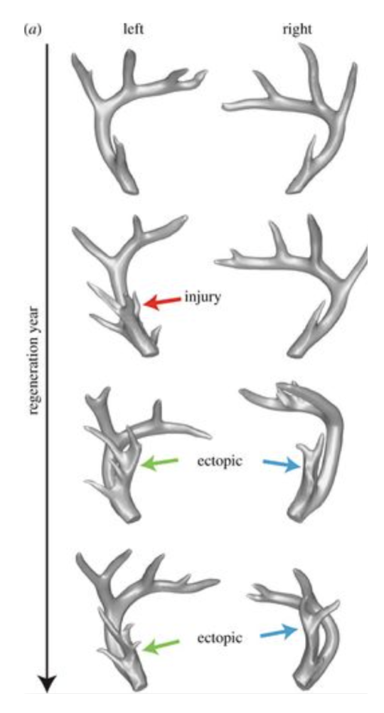
Fig. 9 Deer antlers in three dimensions from a white-tailed buck with trophic memory aged 5 to 8 years (Bubenik & Pavlensky, 1965).

Morphological encodings: a linear encoding

A fundamental assumption of today's molecular genetics is that complex morphology emerges from the simplest encoding. One of the simplest linear encoding types is one-to-one encodings (i.e., direct encodings). As shown in Figure 10, like a blueprint, a one-to-one encoding is formally a bijection: if a function f: A → B satisfies both the injective (one-to-one function) and surjective function (onto function) properties. In other words, each encoding element (domain) is linked with precisely one result element (codomain), and each outcome element is matched with exactly one encoding element (Hammerk, 2018).

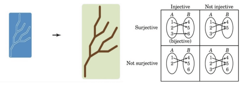
Fig. 10 A one-to-one encoding uses a blueprint to encode the morphology (left) (Lobo et al., 2014), types of functions: injective, surjective and bijective (right) (Hammerk, 2018).

Many organisms follow an isometric (same scale) one-to-one encoding throughout development and regeneration, which is known as a pre-pattern. For example, in Drosophila, the early striped pre-patterns contain morphological information and represent an isometric one-to-one encoding of the larva's potential morphology (Lobo et al., 2014). 

Similarly, Lobo et al. suggested that deer morphology may be described using more complicated linear encodings based on linear mappings between encoding components and result elements. As illustrated in Figure 11, the general linear encoding is based on a string of symbols that are interpreted according to turtle geometry to generate the final morphology: a ‘turtle' that leaves a trace moves according to the sequence of symbols read in the string. The letter ‘F' moves the turtle in a straight line, forming a segment in the morphology, while the symbols ‘+' and ‘-‘ increase or reduce the angle that the turtle is facing, respectively, and the brackets establish a turtle subpath from the present point (Lobo et al., 2014).

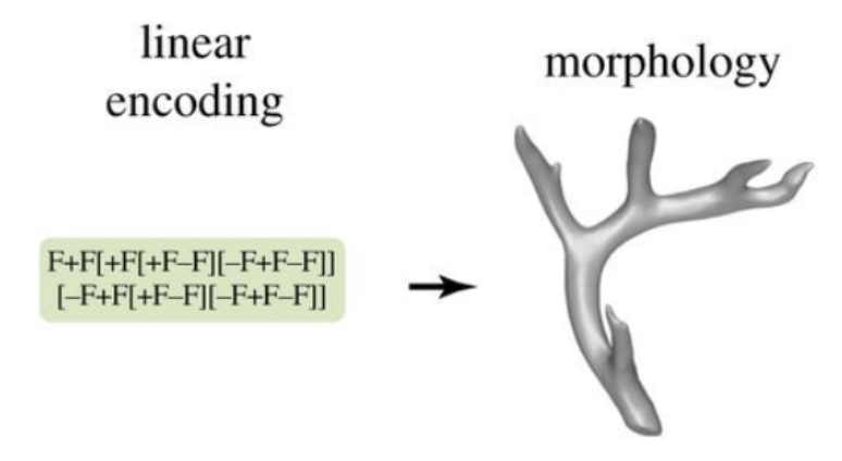
Fig. 11 A linear encoding employs a turtle geometry to convert a string of instructions into the morphology: Every symbol in the string indicates a ‘turtle' leaving a trace in turtle geometry.

Trophic memory and linear encoding

The question is how deer's trophic memory generates ectopic antlers in their next regenerated antlers. As previously stated, when a developing antler is injured, its morphology is modified with a new royal precisely at the location of the trauma. This would be explained by the linear encoding system of the antler morphology. 

Figure 12 depicts how injuries or drugs can disrupt linear encoding locally, resulting in a local change in regenerated morphology. An injury during the development of a tine in a deer antler changes the stored linear encoding precisely at the region where that tine is encoded, resulting in a local variation of the tine's morphology in subsequent regeneration cycles.

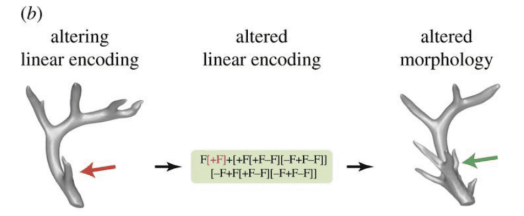
Fig. 12 A lesion to an antler tine (red arrow) can change the encoding of that tine in the code, resulting in regeneration of the antler with a different morphology (a royal, green arrow) exactly where the tine was injured.

Scientists further argued that antler trophic memory is physically placed in the deer nervous system, possibly in the hypothalamus of the brain (Bubenik, 1990). Furthermore, because the antlers are innervated, trauma information can be sent through the neurons in the antlers, which can accurately modify the encoded target morphology in the same location in the following antler cycle (Lobo et al., 2014).

Finally, the finding of morphological linear encodings paved the way for regenerative research. Scientists had trouble interpreting changes in regeneration morphology using a complex nonlinear encoding, but effectively alternating a linear encoding is a considerably easier operation. As a result, this novel perspective on regeneration research utilizing deer antler benefits a wide range of areas, including not just biomedicine but also several computational domains such as robotics.

Analysis of a method for the evaluation and certification of cervid antlers according to a photogrammetry principle using a computer-based modelling system

The approval and classification of deer antlers as trophies is interesting for hunting enthusiasts. The use of antlers as hunting trophies is in further expansion due to the relevant value of biometric data that can be collected from these trophies, which can then be analyzed in geometric morphometry (Rubio-Paramio et al., 2016). To classify antlers according to certain criteria, several innovative methods have been developed to facilitate and accelerate the collection and processing of data.  The two most used tools for data collection are the traditional tape measurement method and the contact measurement method.  The contact measurement method is the most widely used one in 3D biological studies and involves articulated arms capable of obtaining point coordinates on the surface of a measured element (Harvati, 2003; Lockwood, 2002).

Moreover, there are computer programs which greatly facilitate data collection such as the three-dimensional scanner or photogrammetry, especially used in creating biological models. The 3D scanner is based on coordinated digitization techniques, thus representing the most accurate technique in terms of collecting many points on element surfaces (Hennessy, 2002; Fortin et al., 2007; Wang, 2005; Goyal et al., 2012).  The experimental context of measurement can sometimes be complex, making traditional measurement methods difficult to apply in the field, notably since they are only reproducible in a controlled environment.

Thus, another revolutionary technique to collect data has been developed to meet the difficult conditions of studying deer antlers.  This technique, called photogrammetry, is based on taking photographs of the specimen from different angles called “points of view”, making it an inexpensive, low energy and non-time-consuming technique (Baltsavias, 1999; Liu, 2012; Ramos, 2011; Golparvar-Fard, 2011).  A ray is then drawn to connect each of these viewpoints to the points on the observed object.  These rays intersect to form the coordinates of the points in three dimensions.  The precise position of the points is therefore determined by calculating the intersection of several straight lines.  Figure 14 portrays the principle of photogrammetry by illustrating the determination of points from two camera angles.

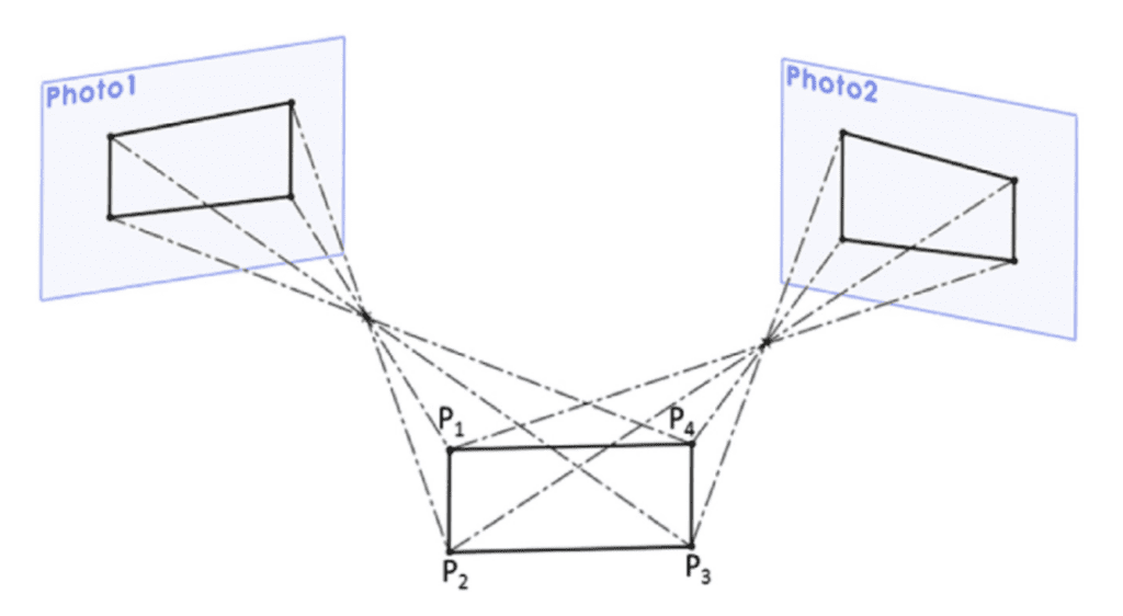
Fig. 13  Determination of the coordinates of different points in space as well as the associated lines starting from two photographic planes having a certain position in three-dimensional space (Rubio-Paramio et al., 2016).

There exists a vector relationship between the coordinates of a point on the object, X_A, and the coordinates of a point on the image, x_a, given by the equation:

\begin{equation}
X_A=X_0-\mu R^tx_a
\end{equation}

Here, X₀ corresponds to the coordinates of the center of perspective 0, representing the focus of the camera, μ is an arbitrary scalar, and where R^t corresponds to the transposed material of the matrix R with the elementary functions of the angle of rotation of the camera. In this case, if the position of the camera X₀ with its angles of rotation is known, then there are three equations and four unknowns, i.e., μ and the three components of the point X_A, which is an impossible system of equations to solve. However, by adding a second camera, a new solvable system is obtained with five unknowns and six equations (Rubio-Paramio et al., 2016).  This new system is illustrated in Figure 14.

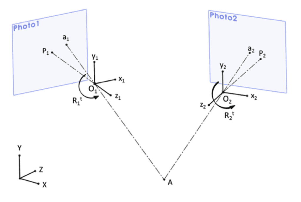
Fig. 14 Determination of the coordinates of points when two cameras are involved in the equation system (Rubio-Paramio et al., 2016).

Typically, photogrammetry information consists of many clustered points where biological elements reconstruction for multiple purposes can be created (Chin-Hung, 2007; Fortin et al., 2007; Shigeta et al., 2013).  This type of model does not always provide the information necessary for its use in biometrics, which is why segmentation techniques based on the observation of elements such as edges, vertices or faces of a 3D model are used to remedy this problem (Demarsin, 2007; Wang & Oliveira, 2007; Wu & Yu, 2005). As for the collection of measurements from deer antlers, it is more complex because experimental situations do not allow taking more than two or three photographs of the specimen, making the reconstruction of the model more difficult.  A method requiring less photographs has been proposed, based on principles of geometric restrictions such as coplanarity, parallelism, perpendicularity, and symmetry (Veldhuis, 1998; Ordonez et al, 2008). 

In practice, the simplest and most effective way of studying the morphology of deer antlers with few landmarks and a significantly reduced number of photographs is to recreate a photogrammetric scene in 3D using a computer-aided system (Rubio-Paramio et al., 2016).  In this sense, a study focusing on developing a new method of branch analysis by reproducing a parametric virtual scene crossed by lines was conducted. This is the interactive photogrammetric measurement method, where only two photographs taken at different angles are required to identify branches that can be formed under adverse conditions (Rubio-Paramio et al., 2016).   In this study, a sample of 29 Iberian red deer antlers were studied under conditions similar to those found in the field to obtain a representative evaluation of the specimens encountered in practice (Rubio-Paramio et al., 2016).  The criteria according to which the branching approval has been carried out are shown in Figure 15.

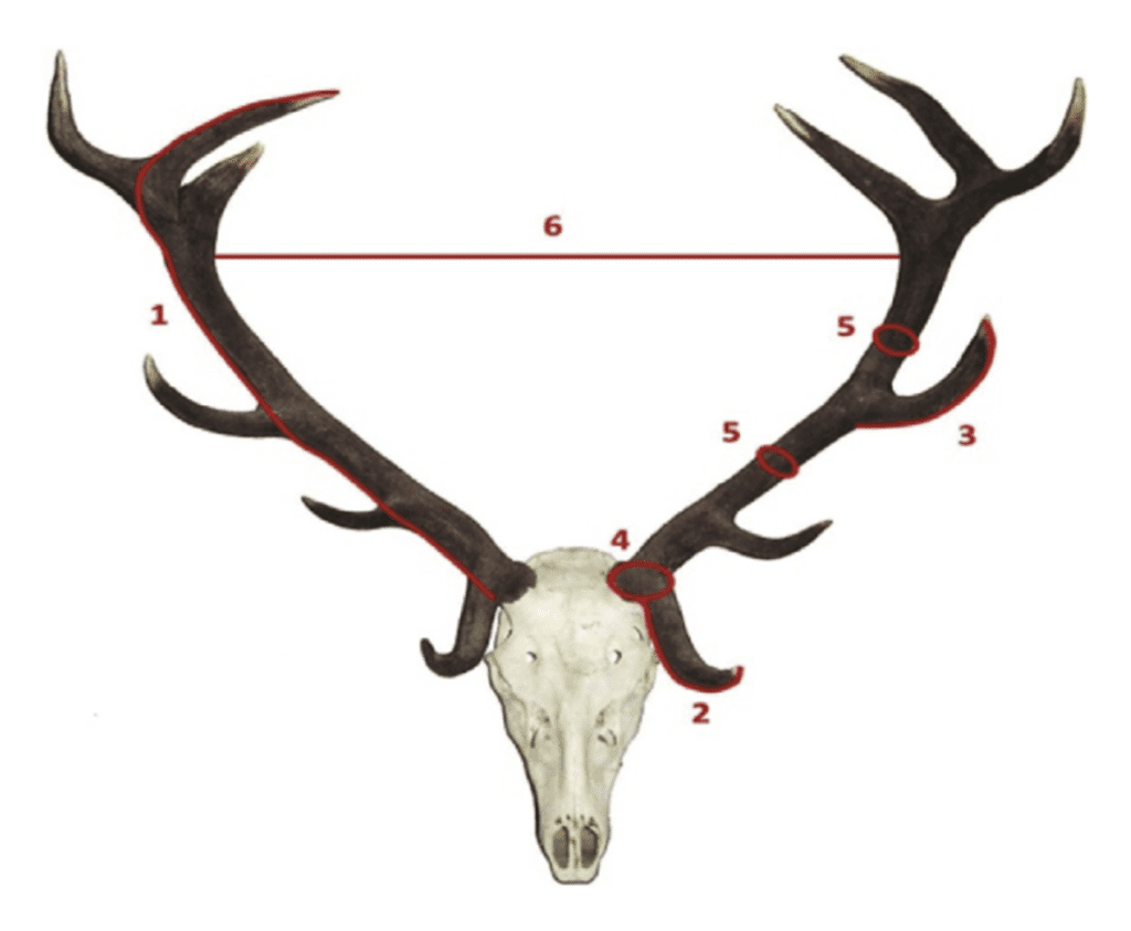
Fig. 15  The different elements of red deer antlers measured during the approval of the antler as a trophy: 1: Length of the main beam of the antler, 2: Length of the tips at eye level. 3: Length of the Trez tips; 4: Perimeter of the burr. 5: Perimeters of certain points of the branch. 6: The maximum internal separation of the branches (Rubio-Paramio et al., 2016).

Let us recall equation (11) illustrated above, i.e.

\begin{equation}
X_A=X_0-\mu R^tx_a
\end{equation}

The interactive photogrammetric method is then based on this equation to represent the lines drawn on the photographs as a structure of parametric lines in a virtual environment. This technique is based on identical landmarks that are found on both photographs, thus facilitating the determination of the points' positions. (Rubio-Paramio et al., 2016). When the photogrammetric method is used, an object with a certain geometry serving as a metric reference is required to reconstruct the antlers of deer (Rubio-Paramio et al., 2016). For instance, a rectangle with all four corners could appear in the photograph, allowing the exact position of the viewpoints to be established, as portrayed in Figure 16.

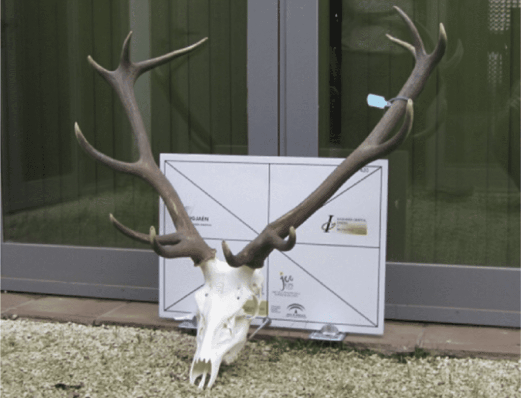
Fig. 16  A metric reference element of a certain size from which lines will be projected to meet at a certain point on an axis perpendicular to the element, i.e., an axis crossing the plane of years in which the element is located (Rubio-Paramio et al., 2016).

From this reference system, it is possible to project lines starting from the reference object that will join at a certain point on an axis perpendicular to the device, revealing the position of the camera. The same process can be replicated for the position of the second camera. Since both photographs have the same reference system, the two scenes can be placed in the same space, such that the lines starting from the two images will overlap, revealing the coordinates of the points forming the outline of the object to be modeled (Rubio-Paramio et al., 2016). Figure 17 illustrates how to achieve this.

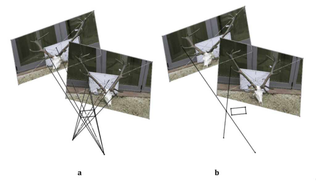
Fig. 17  (a) Superposition of the lines projected from the reference element to the position of the camera, creating a small rectangular area in three-dimensional space, corresponding to the modelled object. (b) Projection of rays from the tip of the antler of a red deer crossing at a specific point in space, i.e. the position of the modeled element (Rubio-Paramio et al., 2016).

Drawing many lines from different points on the two images makes it possible to obtain the actual position of the main branch with its length and curvature, as drawn in Figure 18. The points of intersection of the lines are connected by several curves according to a trajectory recommended by the approval guide, facilitating the measurement of its length afterwards.

Fig. 18 Determination of the actual position of a series of points of intersection between the lines from the two photographs with the curve crossing these multiple points of intersection, revealing the outline of the main branch (Rubio-Paramio et al., 2016).

To obtain the outline of secondary branches in addition to the main branch, the same process as for the main branch is performed. Lines starting from homologous points on the two images are drawn to intersect at a precise position in space, resulting in the modeling of the contour of the entire branch, as shown in Figure 19 (Rubio-Paramio et al., 2016).

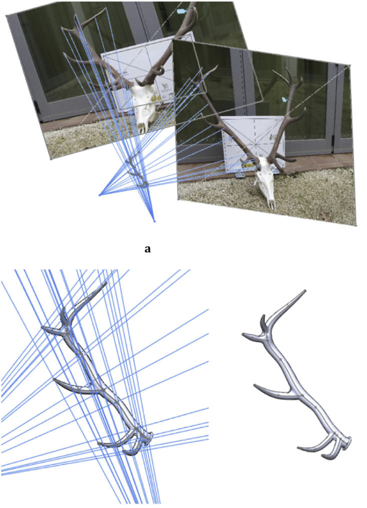
Fig. 19 The extension of thousands of lines from two photographs intersecting at very precise positions allows the creation of a 3D model of red deer antlers from a series of points (Rubio-Paramio et al., 2016).

To give volume to the main branch, small circular planes perpendicular to the curve whose diameter decreases are drawn along the curve from the base to the tip (Rubio-Paramio et al., 2016).   To obtain the branch, the volume passing through all these circular planes was modeled. The tips are modeled in a similar way. As with the main branch, lines starting from the secondary points on the images are crossed to intersect in space to form the outline of the secondary branch.  Small circular planes of different diameters are then drawn at the base, middle and end of the branch and the volume passing through all these circles is modeled. Figure 20 illustrates this technique.

Fig. 20 Creation of the volume of the main branch and secondary branches by drawing circular planes of variable diameter along the contour of the branches (Rubio-Paramio et al., 2016).

Interestingly, this study illustrates all the advantages that the interactive photogrammetry method using an operating system brings to generating deer antler morphology. As a result, measuring with the tape requires many measurements taken by different people or by trained individuals to achieve good results, which is not feasible in practice due to the large number of specimens and difficult conditions. A period of 20 minutes is required to collect the measurements by branching. As for the measurement method with articulated arms, it requires between 30 and 40 minutes to perform, preferably in the laboratory, which is not very efficient compared to the interactive method. The latter requires only 15 minutes and two photographs per branch, allowing to study a large proportion of individuals during data collection. Traditional methods are much more complex than the computer-aided modelling method (Rubio-Paramio et al., 2016). Moreover, the creation of a scene in space from a computerized parametric system allows various photos to be easily adapted, greatly reducing the processing of graphic data following measurements.  Interactive photogrammetry in the modeling of deer antlers is therefore an essential tool to provide important information such as lengths, angles, diameters, or perimeters required for the evaluation of hunting trophies or biometric analyses.

Conclusion

While larger antlers are known to diminish Cervidae longevity of survival in the wild, females perceive them as an indication of possessing superior genes, in accordance with the handicap theory. In other words, while animal ornaments are attractive to the opposite sex, natural selection or survival is at odds with sexual selection. Mathematical models are used to determine the optimal antler size in a population of red deer, allowing males to attract females for mating and win dominance battles without jeopardizing their survival in the wild. Furthermore, antler growth, antler size, casting date, and antler velvet weight are all directly connected to a variety of parameters such as bodyweight, diet, genetics, and age. In experiments, for instance, the date of antler casting is directly proportional to antler weight, and the velvet weight and pre-rut live weight may be described as a linear relationship (y=ax). In some species with regenerative abilities like deer, physical interventions or trophic memory can directly modify the target morphology that their regenerative process restores. Furthermore, linear encoding (i.e., a simple algorithm) can be used to generate the antler morphology, and an injury during the development of a tine in a deer antler changes the stored linear encoding precisely where that tine is encoded, resulting in a local variation of the tine's morphology in subsequent regeneration cycles. Finally, the Interactive Photogrammetric Measure Method (IPhMM) has proven to be a useful device for acquiring appropriate geometric data instantly with only two photographs required per specimen, and this innovative system in deer antler modeling is an essential tool for providing important information such as lengths, angles, diameters, or perimeters that are required for the evaluation of hunting trophies or biometric analyses. Overall, mathematical investigations of the antler regeneration cycle and handicap theory have demonstrated the antler's innovative potential in a variety of domains ranging from biomimetics to regenerative medicine in contemporary society. 

References

Baltsavias, E. P. (1999). A comparison between photogrammetry and laser scanning. ISPRS Journal of Photogrammetry and Remote Sensing, 54(2), 83–94.  https://doi.org/10.1016/S0924-2716(99)00014-3

Bubenik, A. B., & Pavlansky, R. (1965). Trophic responses to trauma in growing antlers. Journal of Experimental Zoology, 159(3), 289–302. https://doi.org/10.1002/jez.1401590302

Bubenik, G. A. (1990). The role of the nervous system in the growth of Antlers. Horns, Pronghorns, and Antlers, 339–358. https://doi.org/10.1007/978-1-4613-8966-8_11

Clements, M.N., Clutton-Brock, T.H., Albon, S.D., Permberton, J.M. & Kruuk, L.E.B. (2010). Getting the timing right: antler growth phenology and sexual selection in a wild red deer population. Oecologia, 164, 357-368. https://doi.org/10.1007/s00442-010-1656-7.

Clifton, S. M., Braun, R. I. & Abrams, D. M. (2016). Handicap principle implies emergence of dimorphic ornaments. Proc. R. Soc. B., 283(1843), 1-6. http://doi.org/10.1098/rspb.2016.1970

Clutton-Brock, T. (2007). Sexual selection in males and females. Science, 318(5858), 1882–1885. https://doi.org/10.1126/science.1133311′ 

Demarsin, K., Vanderstraeten, D., Volodin, T., & Roose, D. (2007). Detection of closed sharp edges in point clouds using normal estimation and graph theory. Computer-aided Design, 39(4), 276–283.  https://doi.org/10.1016/j.cad.2006.12.005

Fortin, D., Cheriet, F., Beauséjour, M., Debanné, P., Joncas, J., & Labelle, H. (2007). A 3D visualization tool for the design and customization of spinal braces. Computerized Medical Imaging and Graphics, 31(8), 614–624.  https://doi.org/10.1016/j.compmedimag.2007.07.006

Golparvar-Fard, M., Bohn, J., Teizer, J., Savarese, S., & Peña-Mora, F. (2011). Evaluation of image-based modeling and laser scanning accuracy for emerging automated performance monitoring techniques. Automation in Construction, 20(8), 1143–1155.  https://doi.org/10.1016/j.autcon.2011.04.016

Goss, R. J. (1983). Deer antlers: regeneration, function and evolution. New York: Academic Press. 

Hammack, R. (n.d.). Book of proof – third edition. Open Textbook Library. Retrieved November 27, 2022, from https://open.umn.edu/opentextbooks/textbooks/7

Harmel, D. E., Williams, J.D., & Armstrong, W.E (1988). Effects of Genetics and Nutrition on Antler Development and Body Size of White-Tailed Deer. https://tpwd.texas.gov/publications/pwdpubs/media/pwd_bk_w7000_0155.pdf

Harvati, K. (2003). Quantitative analysis of neanderthal temporal bone morphology using three-dimensional geometric morphometrics. American Journal of Physical Anthropology, 120(4), 323-338. doi:10.1002/ajpa.10122

Hayden, T. J., Lynch, J. M., & O'Corry‐Crowe, G. (1994). Antler growth and morphology in a feral sika deer (cervus nippon) population in Killarney, Ireland. Journal of Zoology, 232(1), 21–35. https://doi.org/10.1111/j.1469-7998.1994.tb01557.x

Hennessy, R. J., & Stringer, C. B. (2002). Geometric morphometric study of the regional variation of modern human craniofacial form.  American Journal of Physical Anthropology, 117(1), 37-48. doi:10.1002/ajpa.10005

Iten, L. E., & Bryant, S. V. (1973). Forelimb regeneration from different levels of amputation in the newt,notophthalmus viridescens: Length, rate, and stages., 173(4), 263–282. https://doi.org/10.1007/bf00575834

Lande, R. (1981). Models of speciation by sexual selection on polygenic traits. Proc. Natl Acad. Sci., 78, 3721–3725. https://doi.org/10.1073/pnas.78.6.3721

Li, C., Yang, F., & Sheppard, A. (2009). Adult stem cells and mammalian epimorphic regeneration-insights from studying annual renewal of Deer Antlers. Current Stem Cell Research & Therapy, 4(3), 237–251. https://doi.org/10.2174/157488809789057446

Liu, T., Burner, A. W., Jones, T. W., & Barrows, D. A. (2012). Photogrammetric techniques for aerospace applications. Progress in Aerospace Sciences, 54, 1–58.   https://doi.org/10.1016/j.paerosci.2012.03.002

Lobo, D., Solano, M., Bubenik, G. A., & Levin, M. (2014). A linear-encoding model explains the variability of the target morphology in regeneration. Journal of The Royal Society Interface, 11(92), 20130918. https://doi.org/10.1098/rsif.2013.0918

Lockwood, C. A., Lynch, J. M., & Kimbel, W. H. (2002). Quantifying temporal bone morphology of great apes and humans: An approach using geometric morphometrics.  Journal of Anatomy, 201(6), 447-464. doi:10.1046/j.1469-7580.2002.00122.x

McHanon, M (2022). What are the “Points” on a Buck? All Things Nature. https://www.allthingsnature.org/what-are-the-points-on-a-buck.htm

Muir, P.D. & Sykes, A.R. (1988) Effect of winter nutrition on antler development in red deer (Cervus elaphus): A field study. New Zealand Journal of Agricultural Research, 31(2), 145-150.  https://doi.org/10.1080/00288233.1988.10417938.

Nur, N., & Hasson, O. (1984). Phenotypic plasticity and the handicap principle. Journal of Theoretical Biology, 110(2), 275-297. https://doi.org/https://doi.org/10.1016/S0022-5193(84)80059-4 

Ordóñez, C., Arias, P., Herráez, J., Rodríguez, J., & Martín, M. T. (2008). Two photogrammetric methods for measuring flat elements in buildings under construction. Automation in Construction, 17(5), 517–525.  https://doi.org/10.1016/j.autcon.2007.11.003

Pierce, R.A., Sumners, J., Flinn, E. Antler Development in White-Tailed Deer: Implications for Management. Extension University of Missouri. https://extension.missouri.edu/publications/g9486

Ramos, J. B. P., Ferreira, F. A. F., & Barata, J. M. M. (2011). Banking services in Portugal: a preliminary analysis to the perception and expectations of front office employees. International Journal of Management and Enterprise Development, 10(2/3), 188. https://doi.org/10.1504/ijmed.2011.041549 

Rubio-Paramio, M. A., Montalvo-Gil, J. M., Ramírez-Garrido, J. A., Martínez-Salmerón, D., & Azorit, C. (2016). An interactive photogrammetric method for assessing deer antler quality using a parametric Computer-Aided Design system (Interactive Photogrammetric Measure Method). Biosystems Engineering, 150, 54–68.  https://doi.org/10.1016/j.biosystemseng.2016.07.012

Schaffer, W. A. (1983). The Application of Optimal Control Theory to the General Life History Problem. The American Naturalist, 121(3), 418-431. http://proxy.library.mcgill.ca/login?url=https://www.jstor.org/stable/2461159

Shigeta, Y., Hirabayashi, R., Ikawa, T., Kihara, T., Ando, E., Hirai, S., Fukushima, S., & Ogawa, T. (2013). Application of photogrammetry for analysis of occlusal contacts. Journal of Prosthodontic Research, 57(2), 122–128.  https://doi.org/10.1016/j.jpor.2012.11.004

Teng, C.-H., Chen, Y.-S., & Hsu, W.-H. (2007). Constructing a 3D trunk model from two images. Graphical Models, 69(1), 33–56.  https://doi.org/10.1016/j.gmod.2006.06.001

Veldhuis, H., & Vosselman, G. (1998). The 3D reconstruction of straight and curved pipes using digital line photogrammetry. ISPRS Journal of Photogrammetry and Remote Sensing, 53(1), 6–16.  https://doi.org/10.1016/S0924-2716(97)00031-2

Wang, C. C. L. (2005). Parameterization and parametric design of mannequins. Computer-aided design, 37(1), 83–98.  https://doi.org/10.1016/j.cad.2004.05.001

Wang, J., & Oliveira, M. M. (2007). Filling holes on locally smooth surfaces reconstructed from point clouds. SIBGRAPI, 25(1), 103–113.  https://doi.org/10.1016/j.imavis.2005.12.006

Wu, H., & Yu, Y. (2005). Photogrammetric reconstruction of free-form objects with curvilinear structures. The Visual Computer, 21(4), 203–216. https://doi.org/10.1007/s00371-005-0281-7