Exploration of Mathematical Laws Governing Claws and their Applications within Flying Animals, Terrestrial Pests, and Amniotes

Liela Andringa, Alan Fu, Alex Jung, Oscar Cruz Hernandez

Abstract

Claws are one of the most widely utilized tools within organisms, and for a good reason: their purposeful constructions, described by mathematical laws and correlations, allow a wide range of use. This research paper investigates these fascinating mathematical relationships, beginning with the connection between claw growth and logarithmic functions. Applying these mathematical relations, the effect claw curvature has on flying animals, especially concerning predator-prey relations, is shown. Furthermore, this essay dives into the analytical aspects of the intuitive relationship between claw geometry and function using beetles, voles, and amniotes as applicable examples. This essay explores the predictions made about extinct species through mathematical correlations of claw curvature found in an astonishing new field of study. While claw mathematics can be used to analyze the past, it can also be used to pave the way towards the future. In this essay, readers will discover how engineers can model their designs on the mathematics of claws to influence and optimize future projects.

Introduction

Mathematics grants us the ability to quantitatively understand and describe the initially unpredictable habits of nature – furthermore, the universe. The nature of the claw is no exception. 

The claw can be examined through various comparisons to mathematical functions. Specifically, through the analysis of Archimedes' spiral and varying growth rates of the claw, it is found that claw growth shares many structural features with logarithmic functions. The mathematical analysis of claw growth then brings to attention the various ways it can affect flying animals. As a result, claw curvature affects flying animals regarding its role in the ecosystem and their ability to hunt. Furthermore, powerful conclusions can be drawn on the ecological niche of extinct animals through statistical relations between claw curvature and ecological niche. In addition, this paper addresses the relationship between claw geometry and its functions corresponding to beetles and voles as exemplary exhibitions. In both cases, an analysis of the geometry of the curvature of the inner segment of the claw was conducted to find how the variations in that curvature enable the animals' movement and specific uses, from climbing to burrowing, of their claws. Further investigation in claw geometry is done when comparing amniote's claw shapes from other species and its position and function. By modeling the claw with different ratios, one is able to identify the origin of claws and even find the most effective way to model excavation machines which improve digging performance.

This research and mathematical analysis of the claw provides exceptional inspiration for biomimicry towards improving digging technology for mining and agricultural machinery, while also assisting in paleontology and evolutionary biology fields.

Mathematics of claw growth

General background information

Based on biological and physical properties of the keratin protein, the claw grows in a particular shape that can be further analyzed mathematically. The most common growth patterns observed in claws are the logarithmic growth pattern and the power cascade. These two growth patterns greatly influence the shape and functionality of an animal's claw.

To fully comprehend the nature of claw growth, one must first understand the mathematical functions and vocabulary used in determining the claw's relationship with mathematics. This is general background information to help build a foundation of surface level understanding before investigating more complex depths of claw mathematics.

To begin, claw growth can be described to follow a logarithmic growth pattern. The logarithmic growth pattern gets its name because claw growth visually resembles the graph of any logarithmic function. Examples of such functions are presented in Figure 1.

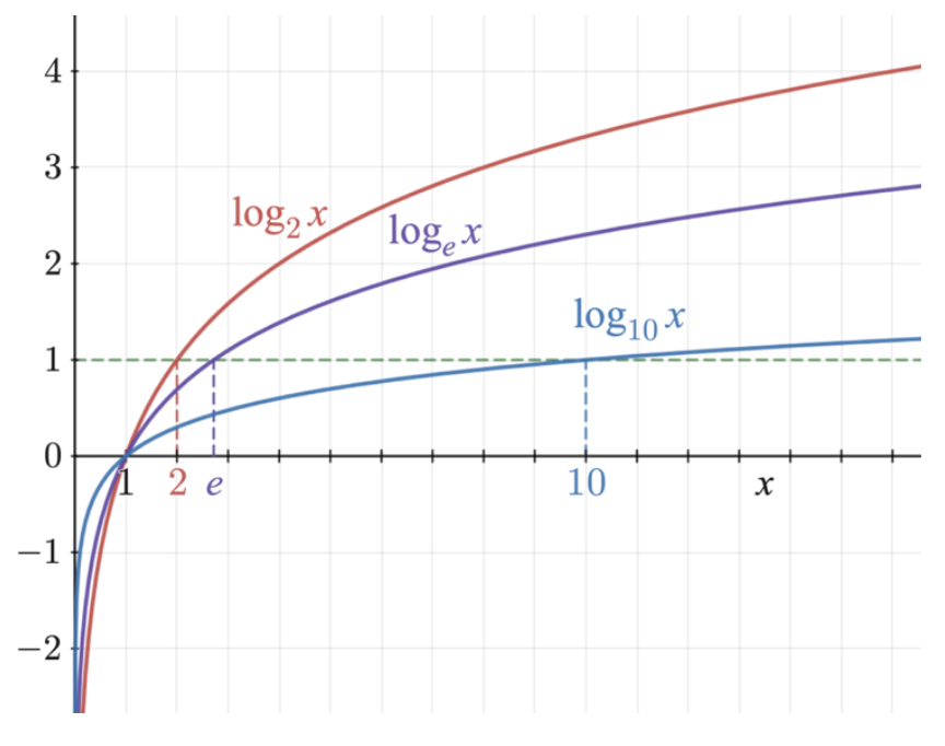
Fig. 1 Logarithmic functions (Adapted from Lyon, 2011).

The logarithmic growth pattern throughout the claws results in a spiral growth trajectory called a logarithmic spiral. A logarithmic spiral (also known as Archimedes' spiral) is a spiral where the radius and the tangential angle both grow exponentially as the function spirals away from its center (Britannica, 2022). The logarithmic spiral is shown in Figure 2.

Fig. 2 Logarithmic Spiral (Adapted from Cook, 2022).

This spiral is represented by Equation 1.

r=a\theta

Eq. 1 Equation for a logarithmic spiral.

Here, r is the radius from the center of the spiral, a is a constant, and θ is the angular position that tracks the number of rotations (Britannica, 2022).

Overall, these two valuable subjects are deeply involved in claw growth and will be helpful concepts to understand while diving deeper into this subject.

Logarithmic growth pattern

The logarithmic growth pattern considers the different growth rates of the base to the tip of the claw (Evans et al., 2021). The formation of a growing claw depends on the growth rates of the unguis and the subunguis of the claw. The unguis is the top portion of the claw that acts as a tough exterior; whereas the subunguis is a ventral plate at the bottom of the claw covered by the unguis (Alibardi, 2016). These two components are annotated in Figure 3.

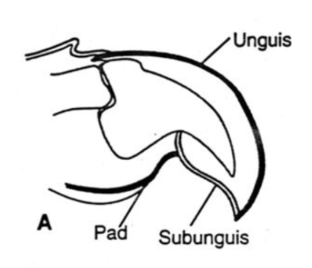
Fig. 3 Diagram of the unguis and the subunguis on a claw (Adapted from Feldhamer et al., 2004).

Depending on the growth rate of each of these components, they create the curvature of the claw. To clarify, if the growth rates of the unguis and the subunguis are equivalent, the claw maintains a conical shape with no curvature in any direction. However, if the claw components in question were to grow at different rates, the claw would start to create a curved structure leaning towards the side with the slower growth rate (Evans et al., 2021). The growth rate of the unguis will always be larger or equal to the growth rate of the subunguis because the unguis needs to curl over the subunguis since it has a durable protective shell. A visualization can be found in Figure 4, where different growth rates of the unguis and the subunguis are tested and compared to a logarithmic spiral.

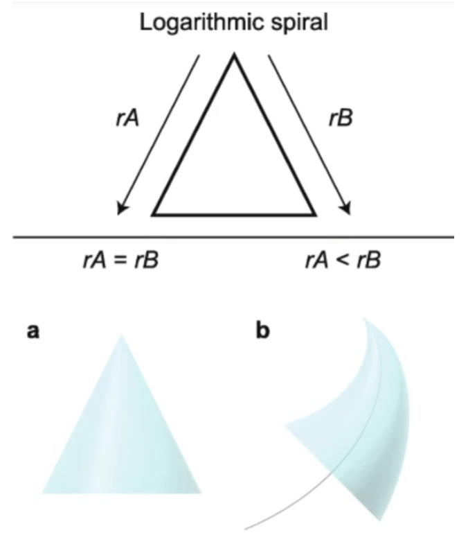
Fig. 4 Logarithmic growth pattern examples (Adapted from Evans et al., 2021).

As shown in Figure 4 structure (a), the growth rate of the unguis (rB) and the growth rate of the subunguis (rA) are equal, which results in a cone-like structure. In Figure 4 structure (b), growth rates rA and rB are unequal, creating a curved shape known as the logarithmic spiral (Evans et al., 2021). The larger the difference in the growth rates of the unguis and the subunguis, the more intense the curvature of the claw becomes. Therefore, the logarithmic growth pattern explains the relationship between the curvature of the claw and its growth rates.

Power cascade

Another concept heavily involved in claw growth patterns is the power cascade. The power cascade relies on the power growth rate of the claw length and the growth rate of the claw's radius (Evans et al., 2021). The power growth rate of the claw length is the growth rate considering the arc length of the claw, while the growth rate of the radius is the change in radius (of the vertical cross-section of the claw) over time. When these two rates are equivalent, the claw takes a conical shape with zero curvature, similar to structure (a) in Figure 4. To better explain the power cascade, below in Figure 5 are examples of different types of power cascades. Furthermore, this figure shows that the logarithmic spiral and the power cascade work together to influence the shape of the claw.

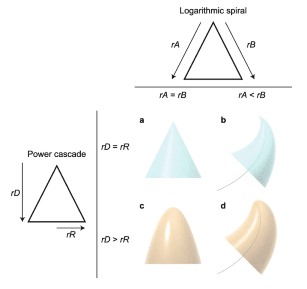
Fig. 5 The effect of the logarithmic spiral and the power cascade in claw shape (Adapted from Evans et al., 2021).

As presented in Figure 5, if the growth rate of the radius (rR) is less than the growth rate of the length (rD), then the claw forms a conical shape similar to a 3D parabola known as a power cone, as shown in structure C. A power cone is created whenever rR and rD are unequal. Finally, structure D from Figure 5 can be analyzed. This structure is created by incorporating the inequality of both growth rates of the logarithmic spiral and the power cascade. Therefore, structure D's shape is generated when rA < rB (which creates a logarithmic spiral trajectory) and rD > rR (which creates a power cone). This creates a new structure called a power spiral where the power cone is curved on a logarithmic spiral trajectory (Evans et al., 2021). 

Overall, the logarithmic spiral is responsible for creating the claw's curved shape; whereas the power cascade is responsible for forming the claw's shape in volume (length and width). Knowing these mathematical techniques in describing claw growth and curvature, researchers can use these methods to analyze different claw shapes in various species. This will allow us to further understand the most effective claw shapes for a variety of functions used by many different species of animals.

Claw mathematics in flying animals 

Claw curvature in relation to ecological niche

The topic of the original evolution of flight within animals has been a debate among paleontologists for centuries, and for good reason: the ability of an animal to balance four different forces of lift, weight, thrust, and drag in their favor to soar into the sky is arguably one of the most impressive locomotive capabilities of animals today. Even with the discovery of the Archaeopteryx, the oldest known bird, shown in Figure 6 below, the answer to the question of flight evolution eludes us, despite it having evolved at least four times independently in birds, bats, insects, and pterosaurs (an extinct clade of flying reptiles). 

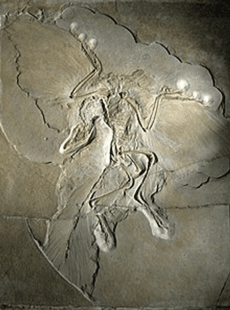
Fig. 6 An original Archaeopteryx fossil displayed at the Museum für Naturkunde in Berlin (Adapted from Wikipedia, Courtesy of H. Raab, 2009).

Paleontologists have postulated many theories, from arguing that flight evolved from the ground up to flight evolving in arboreal animals that leaped down from trees to wings evolving to assist with incline running and eventually achieving flight. One novel way paleontologists have used to research this phenomenon is to connect the mathematical properties of claws to the ecological niches of birds to project this approach onto extinct species like the Archaeopteryx. This approach is effective because the bony cores of claws in fossils are well-preserved through time. While studies mainly focus on analyzing the keratinous sheaths of claws, a strong correlation has been noted between the keratinous sheaths and bony cores of claws, as seen in Figure 7 (Hedrick et al., 2019).

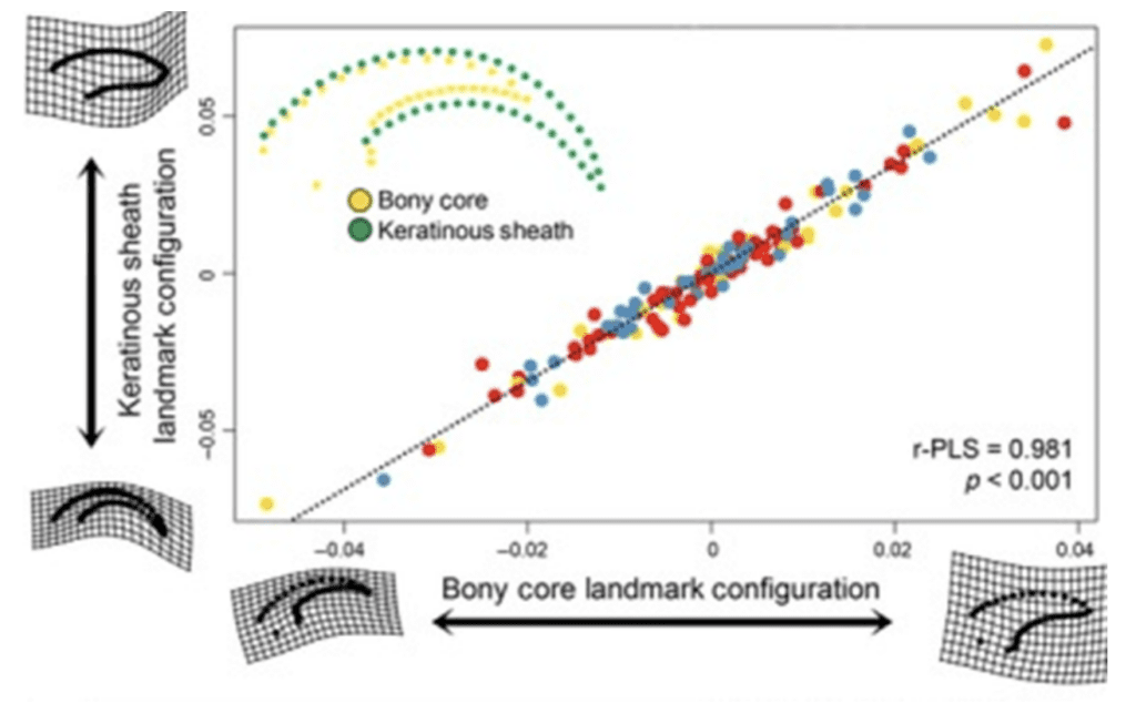
Fig. 7 Analysis of bony core and keratinous sheath landmark configurations using two-block partial least squares regression where blue represents predatory birds, red represents flying birds, and yellow represents ground birds (Adapted from Hedrick et al., 2019).

This study noted a significant correlation between the bony core and keratinous sheath of bird claws, with a p-value less than .001, enabling this mode of study. Researcher Alan Feduccia was one of the first to dive into this field of study, examining over 500 species of birds and categorizing them according to their ecological niches as ground-dwellers, perchers, and climbers in order to examine patterns within the angle of the inner curvature of the claw. We see the method of study in Figure 8.

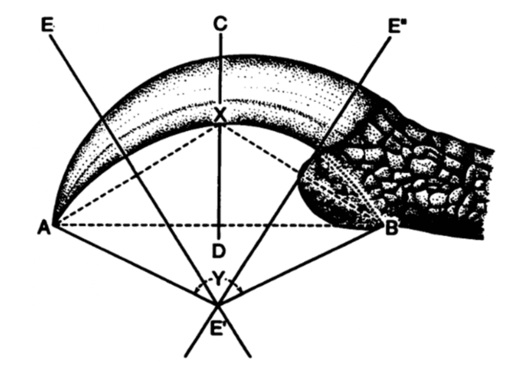
Fig. 8 Measure of the angle of inner curvature of a claw (Y) through multiple chords and perpendicular (Adapted from Feduccia, 1993).

There was a significant separation between the claws of ground-dwelling birds and other birds; the inner curvature angle of ground-dwelling birds averaged 64.3°, compared to a perching bird mean of 116.3° and a climbing bird mean of 148.7°. A one-way analysis of variance between these three groups was significant at P < 0.001, as can be seen indistinction between these groups in Figure 9.

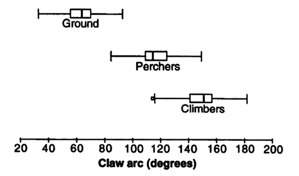
Fig. 9 Box and whiskers plot of inner curvature claw arc of ground-dwelling, perching, and climbing birds (Adapted from Feduccia, 1993).

The Archaeopteryx's claws had a mean measurement of 120°. While there was an overlap between the inner curvature angles of perching and climbing birds, this study notes the possibly arboreal nature of the Archaeopteryx's ecological niche. However, comparisons with modern birds did not hold the same results. The Australian pheasant cuckoo, Centropus phasianinus, displays an incredible similarity in morphology to the Archaeopteryx, as shown in Figure 10.

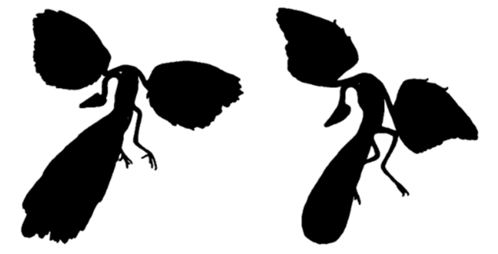
Fig. 10 Silhouettes of the Archaeopteryx (right) and the Australian pheasant cuckoo (left) (Adapted from Feduccia, 1993).

However, despite this remarkable near-mirroring, measurements of the inner curvature angle for the Australian pheasant cuckoo leave it with an average of 85.7°, placing it securely within the range of ground-dwelling birds, in contrast to the Archaeopteryx. These inconclusive results created the need for further research into these connections, thus leading to this branch of paleontology.

In body form and body proportions, the Archaeopteryx is most similar to modern birds like turacos, chachalacas, and Cuculiformes, an order consisting of small to medium-sized birds like cuckoos and hoatzins. Glen and Bennett decided to compare Cuculiformes with Columbiformes, an order consisting of birds like pigeons and doves, to draw further conclusions on the evolution of flight by examining the ecological niches of Mesozoic birds like the Archaeopteryx. Furthermore, they decided to drop classifications like ground-dwelling, perching, and climbing in favor of categorizing birds based on the amount of ground-foraging and tree-foraging behavior. While they took a different approach of deciding to measure the angle of outer claw curvature in contrast to the methods of Feduccia, as shown in Figure 11, other studies have noted a strong correlation between the angle of inner and outer claw curvature (Birn-Jeffery, 2012).

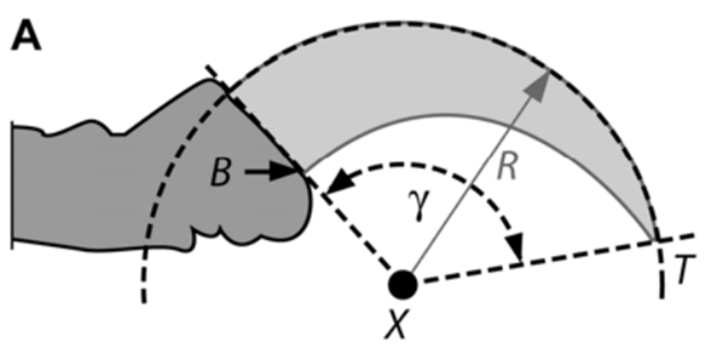
Fig. 11 Measurement of outer claw curvature angle (γ) (Adapted from Glen & Bennett, 2007).

This study recorded outer curvature claw angles of 81 for Columbiformes species and 62 for Cuculiforme species, with a total of 451 specimens examined. Based on times spent foraging on the ground and in trees, the birds were classified as either ground-based foragers (GB), dedicated ground foragers (Gg), predominantly ground foragers (Ga), predominantly arboreal foragers (Ag), dedicated arboreal foragers (Aa), and vertical-surface foragers (V). A notable positive correlation between arboreal foraging time and outer claw curvature angle was found, as shown in Figure 12, along with differences in mean outer claw curvature angle between all paired tests of groups besides dedicated vs. predominantly ground foragers and dedicated vs. predominantly arboreal foragers, with P less than 0.001.

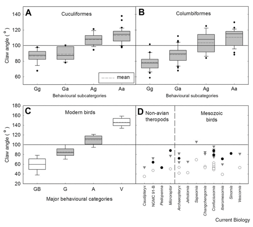
Fig. 12 Box plots of claw angle against behavioral subcategories for Cuculiformes, Columbiformes, and modern birds together, as well as claw angles for several notable Mesozoic birds and non-avian theropods, including the Archaeopteryx (Adapted from Glen & Bennett, 2007).

Notably, there is an apparent increase in claw angle as behavioral subcategories move from primarily ground-foraging species to primarily arboreal-foraging species, with the most significant correlation between the outer claw curvature angles of Gg and Ga as well as Ag and Aa, which is understandable given these pairs' similar behaviors. Furthermore, the placement of the many non-avian theropods and Mesozoic birds almost all fall firmly within the ground-foraging side of the spectrum. This suggests that arboreal foraging likely evolved later and that the ecological niche of these flight-developing theropods and Mesozoic birds lies on the ground, supporting the ground-up and wing-assisted incline running hypotheses.

Indeed, a later study in 2012 by Birn-Jeffery et al. indicated support for some of these conclusions while providing a more comprehensive analysis of claw curvature, analyzing both inner and outer claw curvature angles and comparing them to allometry (bird size). Birds were categorized into groups similar to Feduccia's, with ground-dwellers, perching, climbing, and predatory birds analyzed. Similar results were reported for ground-dwelling, perching, and climbing bird inner and outer claw curvature angles. However, predatory birds seemed to defy this pattern, likely due to the additional use of their claws for hunting, as seen in Figure 13.

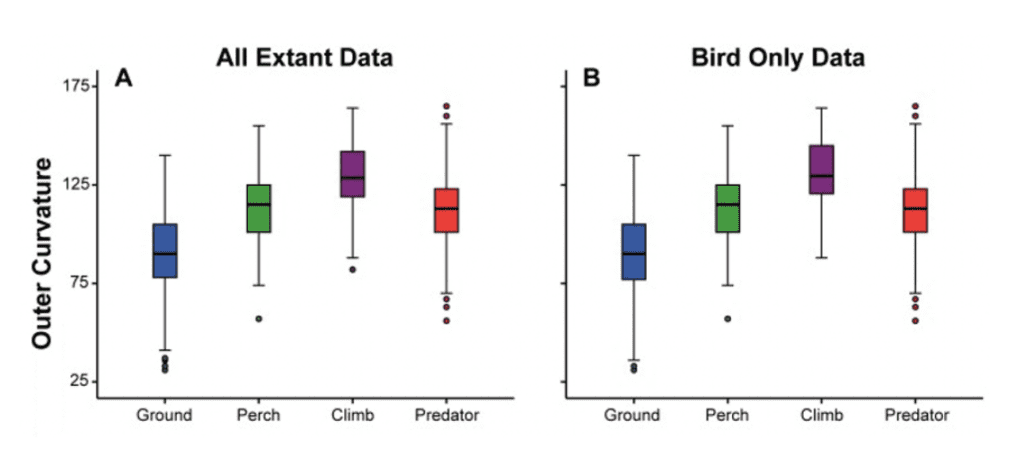
Fig. 13 Box plots for outer claw curvature angle for all extant taxa (A) and extant birds only (B) against ecological niche, and for all extant taxa (C) and extant birds only (D) against relative claw midpoint height (Adapted from Birn-Jefferey et al., 2012).

Measuring over 832 specimens of 331 species, the study by Birn-Jeffery et al. in 2012 found a less substantial but still present correlation between ecological niche and outer claw curvature angle. More importantly, they noted that almost all (19 out of 22) Mesozoic birds fell within the ground-dwelling bird category. Despite the overlap between different ecological niches, they discovered significant evidence for the ecological niches of Mesozoic birds.

These statistical analyses of ecological niches with respect to claw curvature provide compelling evidence for use of developmental theories for the evolution of capabilities such as flight, allowing for the classification of the lifestyle of extinct birds through only the remaining bony cores of their claws. However, the debate on the evolution of flight continues due to studies providing contradictory information in other arguments. It remains to be seen whether paleontologists will ever be able to conclude the origin of flight.

Claw curvature and shape in relation to prey

Although claw curvature proves to be a strong predictor of ecological niche for foraging birds, this estimator breaks down when predatory raptors are introduced into the analysis. However, separating these raptors into different orders and noting the hunting methods and prey size, a similarly powerful mathematical correlation can be found between claw curvature and shape to prey and hunting methods.

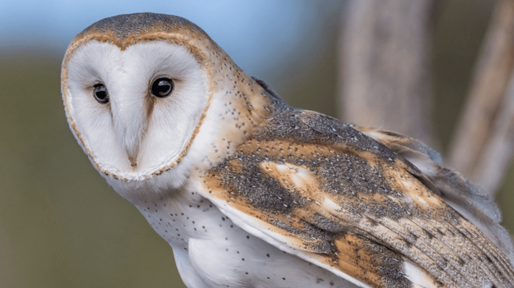
Fig. 14 Barn Owl (Adapted from Audubon Society, Courtesy of Shlomo Neuman, 2014).

Csermely and Rossi in 2006 studied the difference between the claws of birds of prey and non-raptorial birds, using 44 species of Falconiformes (such as falcons), 17 species of Strigiformes (such as owls), and 80 non-raptorial species. Measurements were done on the back claw (D-I) and the front middle claw (D-III). Through fourteen different measurements on ratios of height, width, curvature, and radius of the claws, a Discriminant Function Analysis was performed to obtain the graph shown in Figure 15.

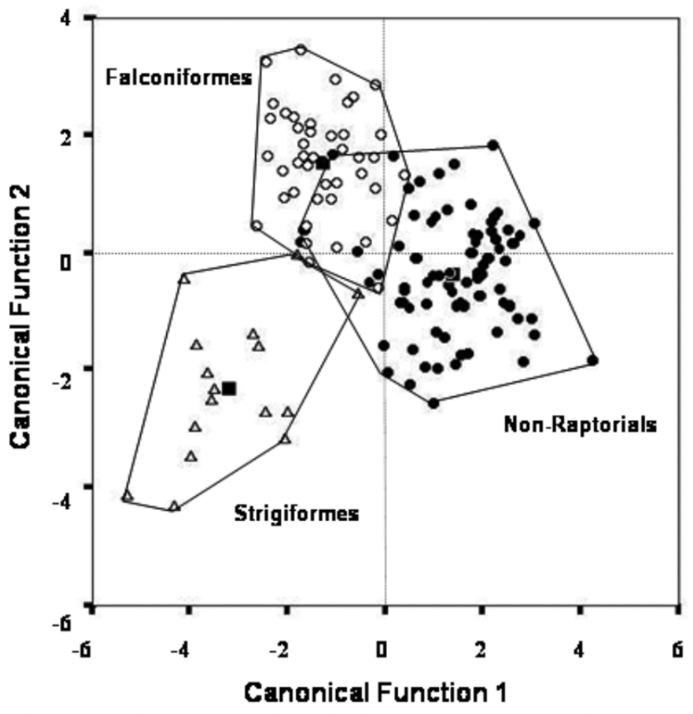
Fig. 15 Plots of two canonical variables relating fourteen ratios of height, width, curvature, and radius of Falconiformes, Strigiformes, and non-raptorial claws (Adapted from Csermely & Rossi, 2006).

The first canonical discriminant function separates non-raptorial birds from Strigiformes and Falconiformes, while the second canonical discriminant function, despite separating Falconiformes and Strigiformes, fails to distinguish non-raptorial birds. However, despite the overlap between non-raptorial birds and Falconiformes, few species of non-raptorial birds fall within the overlap area. Notably, the overlap area mainly consists of the lightest Falconiformes, such as Falconidae, and the heaviest non-raptorial birds, such as corvids. Nevertheless, it can be concluded that there is a clear distinction between non-raptorial bird species and raptors, and it remains to determine the inner workings of this distinction.

Indeed, Tsang et al. (2019) reported similar findings of non-predatory birds having shorter claws and lower curvature, as illustrated in Figure 16 below. The size of the prey is determined by whether the prey fully fits a raptor's claws (medium), is too small to fully fit (small), or is too large to fully fit (large).

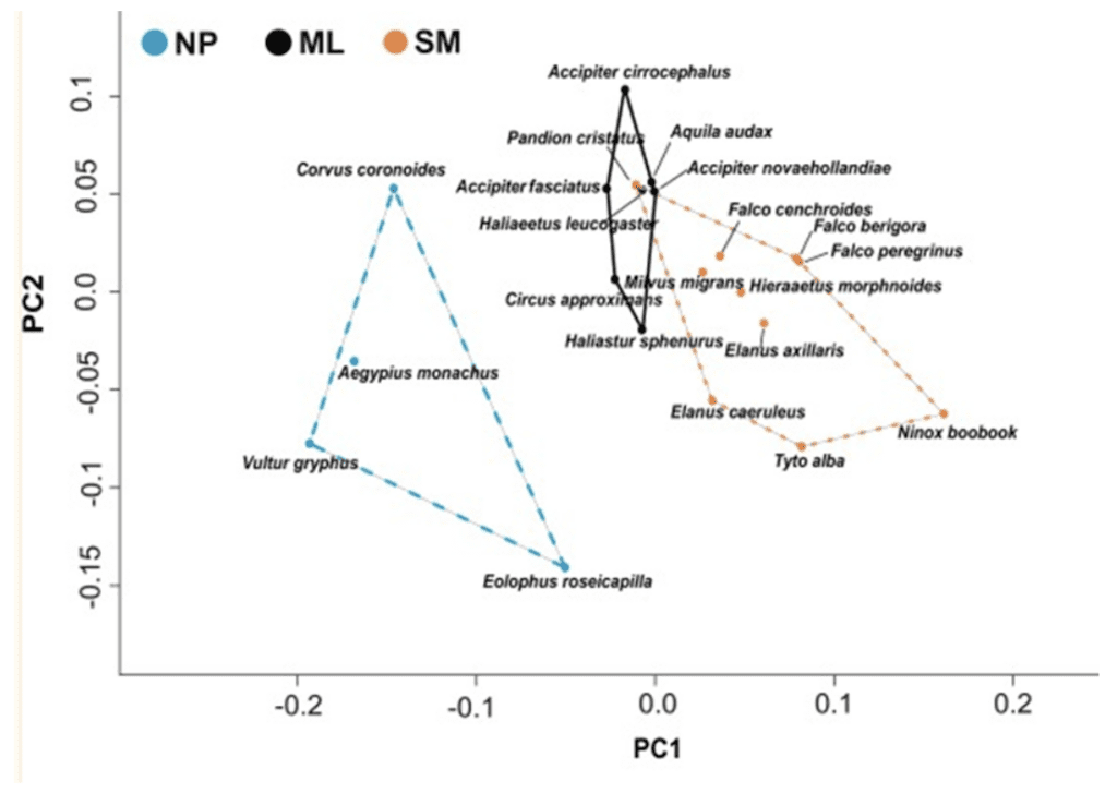
Fig. 16 Plot of nonpredator (NP), medium to large diet raptors (ML), and small to medium diet raptors (SM) in a principle component analysis, where PC1 indicates curvature and PC2 indicates prey size (Adapted from Tsang et al., 2019).

There is a clear distinction in curvature in non-predatory birds compared to predatory birds, supporting the conclusion that there is strong curvature in raptors due to their need for claws in hunting. Furthermore, the ability to withstand stress also changes based on diet, likely as a result of raptors requiring their claws to withstand high amounts of stress from the struggles of prey in order to capture their food. As expected, raptors that prey on medium to large food items have the lowest mean von Mises (VM) stress values, whereas non-predatory birds have the highest, as shown in Figure 17.

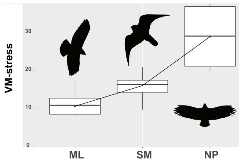
Fig. 17 Boxplot of mean VM stress values for medium to large diet raptors (ML), small to medium diet raptors (SM), and non-predatory birds (NP) (Adapted from Tsang et al., 2019).

An ANOVA test showed significant results with r² = .568 and a p-value ≈ .001. Notably, the osprey, with its highly curved claw, exhibited abnormally high VM stress values compared to other birds in the SM category, likely due to its specialized piscivorous diet requiring slender claws to pierce fish. VM stress values provide another point of analysis in the relation of prey to claw shape. However, deeper categorization of prey and raptor order is needed to grasp this relation fully.

An important point of analysis is the prey which a raptor's claws are intended to capture and kill. Most raptors prefer grasping prey that fully fill their feet to best pierce and penetrate their prey (Cade, 1982). As such, most raptors target prey according to their size, leading to a correlation between raptor size and the size of their main prey (Bouchner, 1977). Fowler et al. (2009) studied three main families of raptors: Falconidae, Accipitridae (such as the bald eagle), and Pandionidae (such as the osprey), along with Strigiformes. Clean breaks between different birds are shown in a correspondence analysis of relative claw sizes shown in Figure 18.

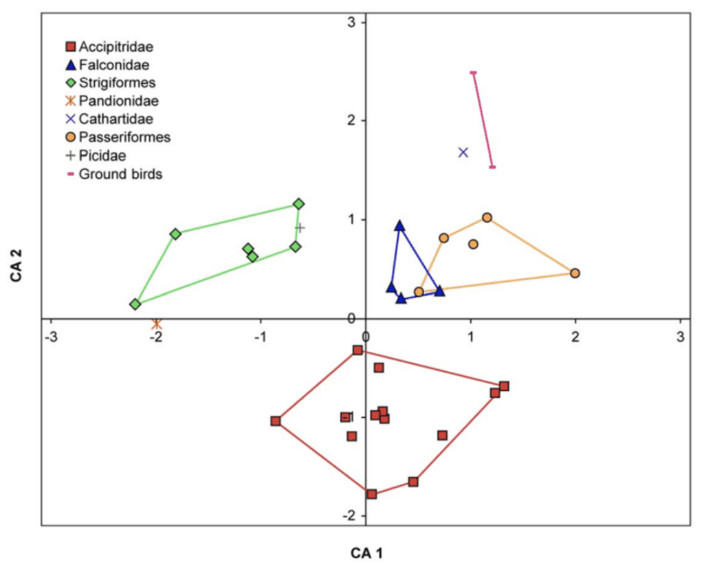
Fig. 18 Correspondence analysis of relative claw sizes among several different taxa. CA 1 is controlled by the sizes of all claws relative to D-III. Axis 2 is controlled by the sizes of claws D-I and D-II (front inner claw) relative to D-IV (front outer claw) (Adapted from Fowler et al., 2009).

There are sharp differences between different taxa, with only a small amount of overlap between Pandionidae and Falconidae. Further exploring this data, Accipitrids have the largest D-I and D-II claws compared to all other taxa, which are very useful for maintaining their grip on large prey when trying to pin down the prey through their body weight. However, only some of their claws are hypertrophied, likely owing to the inclusion of small prey in their diet.  

Strigiformes distinguish themselves from other taxa with their near-uniform, large claws with lower curvature with a mean of 92.256°, as compared to an Accipitridae, Falconidae, and Pandionidae with mean of 112.823°, with a significance of p = 0.002. As Strigiformes only feed on small prey that easily fit into their claws, they rely on constriction to kill them, leading to their enlarged, weakly curved talons. The larger size of the claws compensate for the low curvature, enabling them to maintain the reach of their claws still. 

Falconidae have elongated D-III claws but are otherwise inseparable from passerine claws. Due to a different hunting strategy, Falconidae do not require as many large claws as Accipitridae or Strigiformes. While Strigiformes and Accipitridae kill by ambush and thus require better gripping capabilities, Falconidae kill through strike impact and thus are not as dependent on their gripping capabilities to hunt.  

Pandionidae have highly curved claws, with an outer curvature angle mean of 166° and an inner curvature angle mean of 155.9°, and all of their claws are sub-equally sized. This is due to their specialized piscivorous diet, as hunting fish requires piercing the prey with the claw, leading to an extreme curvature.  

The strong impact of the predatorial lifestyle and, more specifically, in prey choice on claw curvature, shape, and VM stress values is evident. From this information, many conclusions can be extracted on the unknown lifestyles of extinct raptors based on similar methods of analyzing well-preserved bony cores, providing a great asset to paleontology.

Claw mathematics in terrestrial pests

Mathematical modeling of insect claws

Within the class of insects, there are many different creatures with fascinating claws and many reasons for using such appendages. Most insects, however, use their claws for locomotion, being able to crawl on especially rough terrain or inclined surfaces. One of these such insects is the Cyrtotrachelus buqueti Guer, shown in Figure 19. These beetles, considered invasive pests, are found in bamboo forests, scaling and damaging the vertical shoots (Yang, et al., 2017). Although the harm done to the health of the bamboo forests of their habitats is grave, the claws that facilitate their movement along the steep shoots of bamboo are fascinating.

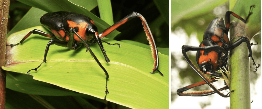
Fig. 19 Cyrtotrachelus buqueti Guer (left) (Adapted from Horstman, 2013) and Cyrtotrachelus buqueti Guer scaling bamboo shoots and inflicting damage (right) (Adapted from Horstman, 2013).

In a study by the Xuzhou University of Technology, researchers analyzed the mechanisms enabling these beetles to traverse such sheer slopes (Li et al., 2022). The researchers initially focused on the adhesion forces between the beetles' claws and the bamboo shoots, finding that it reached at least 67 times the beetles' own weight. Although adhesion forces contribute to their mobility, the geometric features of these beetles' claws are equivalently important. Therefore, the researchers built a mathematical model of the claw of the Cyrtotrachelus buqueti Guer to explore the relationship between the geometric structure and ultimate function of the claw (Li et al., 2022). 

Using scanning electron microscopy (SEM) imaging improved twice over by the image processing algorithms (which denoise an image by evaluating the existing pixels along with their locations in the image and estimating new pixel values along with their locations in the image to produce a more accurate arrangement of pixels), the original non-local means (NLM) algorithm and the improved NLM algorithm, the researchers constructed a solid, relatively clear image of the claw of Cyrtotrachelus buqueti Guer (Kang & Kim, 2021). Edge detection operators were applied to this image to extract the claw edge for implementing feature-curve models. The most effective edge detector (a multi-scale edge detection algorithm) was based on B-spline wavelets. This edge detection operator yielded the clearest claw edge imagery with the least amount of discontinuities or erroneous boundaries. With these denoising algorithms and edge detection operators, the researchers improved the accuracy of boundary information presented in the finalized image of the claw, shown in Figure 20 (Li et al., 2022).

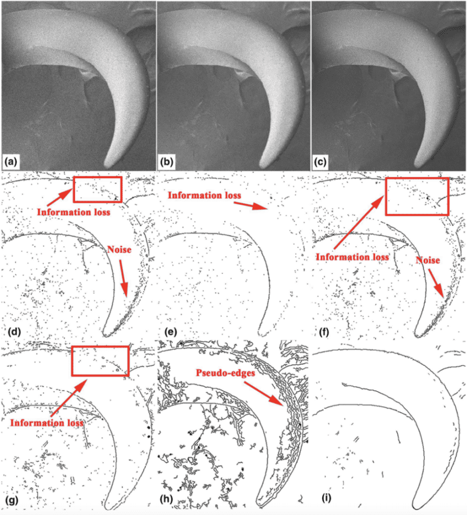
Fig. 20 Imaging of the claw of Cyrtotrachelus buqueti Guer: (a) original SEM image, (b) image improved by NLM algorithm, (c) image further improved by improved NLM algorithm; edge detection of the claw of Cyrtotrachelus buqueti Guer: (d, e, f, g, h) images produced by edge detection of various other operators, (i) finalized image produced by edge detection operator based on B-spline wavelets (Li et al., 2022).

To fit the claw feature curves, researchers used a least squares method, which minimizes the sum of the squares of the differences between the original data points yi and the fitting data points yi, as described by Equation 2. In Equation 2, Φ represents a function class, g(x) represents an arbitrary function in function class Φ, and g^*(x) represents a sought-after function in function class Φ (Li et al., 2022).

\sum_{i=1}^n \left[ g^*(x)-y_i\right]^2=\sum_{i=1}^m\left[g(x)-y_i^2\right]

Eq. 2 Equation for minimizing the sum of the squares of the differences between the original data points and the fitting data points.

The researchers used the coefficient of determination R², described by Equation 3, to evaluate the accuracy of the claw feature curve fitting. High fitting precision is indicated by values of R² close to 1. Here, the residual sum of squares (RSS) and the total sum of squares (TSS) are described by Equation 4 and Equation 5, respectively (Li et al., 2022).

R^2=1-\frac{RSS}{TSS}

Eq. 3 Equation for the coefficient of determination.

RSS=\sum_{i=1}^n(y_i-\dot{y}_i)^2

Eq. 4 Equation for residual sum of squares.

TSS=\sum_{i=1}^n(y_i-\bar y_i)^2

Eq. 5 Equation for total sum of squares.

Researchers decomposed the claw into increasingly intelligible components, developing more clearly defined claw curvature boundaries. Shown in Figure 21 is the comparison of the denoised SEM image of the claw (a), the contour boundary curves extracted from that image (b), and the characteristic curves fitted to those boundaries (c). Four characteristic curves were used to divide the claw to improve the fitting accuracy since each segment of the claw maintains distinct features. To fit the geometrical characteristics of the claw, the researchers used four different functions: a second-order Gaussian function, a second-order Fourier function, a second-order polynomial function, and a third-order polynomial function. The values for the RSS and the R² of each of the four characteristic fitting curves generated by the four different functions are shown in Table 1 (Li et al., 2022).

Fig. 21 Comparison of (a) the denoised SEM image of the claw, (b) the contour boundary curves extracted from that image, and (c) the characteristic curves fitted to those boundaries (Li et al., 2022).

Table 1 Values of the RSS (represented here as SSE) and R² values for each of the four characteristic fitting curves generated by the four different functions (Li et al., 2022).

Considering that the highest fitting precision appeared from the second-order Fourier function, whose R² values were all closest to equaling 1, the researchers used the Fourier function, given by Equation 6, for their calculations of the claw's curvature. The explicit Fourier function used is shown by Equation 7. The Fourier function equation coefficients that were found are shown in Table 2 (Li et al., 2022).

f(x)=a_0+\sum_{i=1}^n(a_i\cos\cos(ixw)+b_i\sin \sin(ixw))

Eq. 6 Equation for Fourier function.

f(x)=a_0+a_1\cos \cos(xw)+b_1\sin \sin(xw)+a_2\cos \cos(2xw)+b_2\sin \sin(2xw)

Eq. 7 Equation for explicit Fourier function.

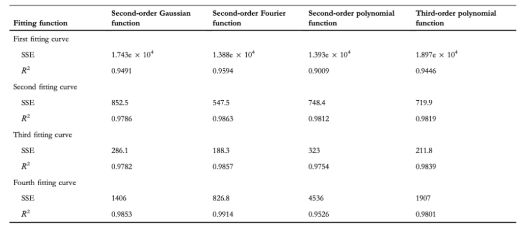
Table 2 Equation and equation coefficients for the fitting claw feature curves (Li et al., 2022).

According to the feature-curve fitting equation, the curvature K can be calculated using Equation 8 (Li et al., 2022).

K=\frac{\lvert y'' \rvert}{(1+y'^2)^{\frac{3}{2}}}

Eq. 8 Equation for curvature of the claw.

Here, y' and y'' represent the first and second derivatives of the fitted curve, respectively. The graphs of the second derivatives of the fitted curve for each of the four characteristic curves of the claw are shown in Figure 22. The graphs of the curvature variations of the fitted curve for each of the four characteristic curves of the claw is shown in Figure 23 (Li et al., 2022).

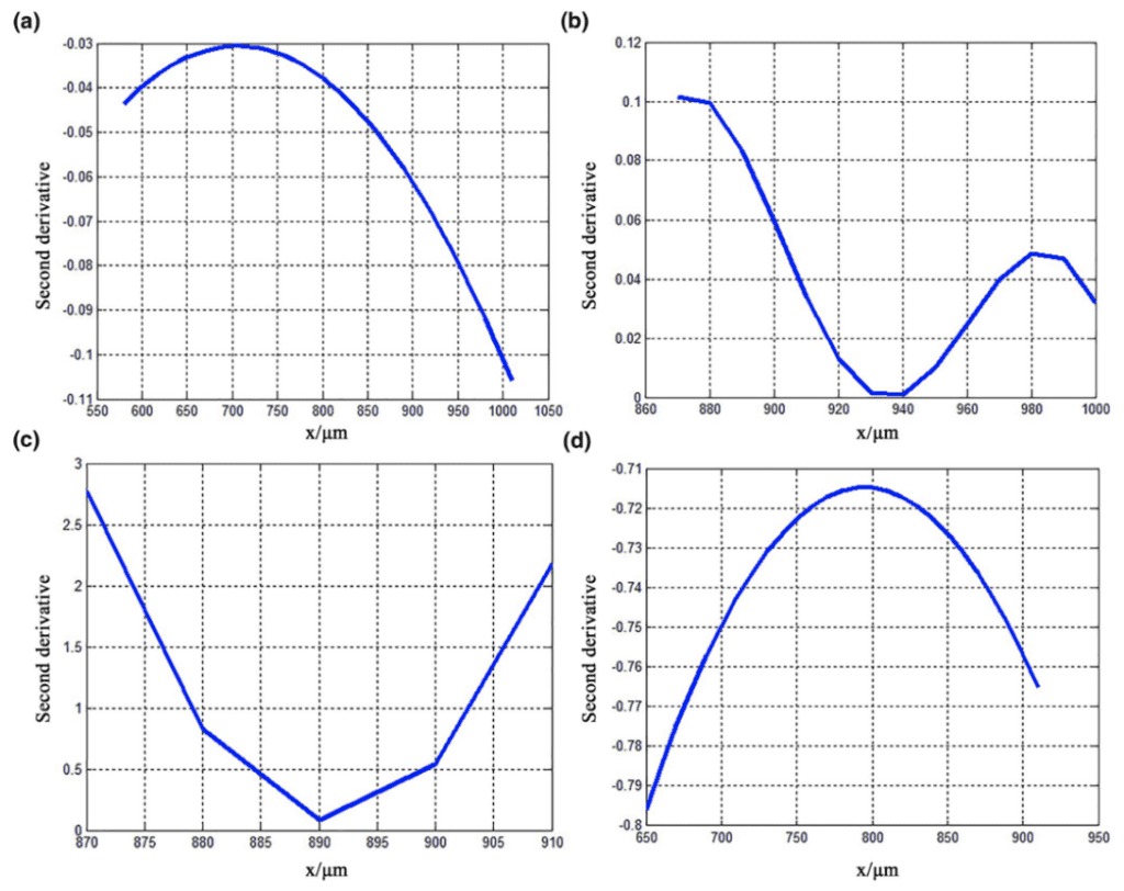
Fig. 22 Graphs of the second derivatives of the fitted curve for the characteristic curves (a) 1, (b) 2, (c) 3, and (d) 4 (Li et al., 2022).

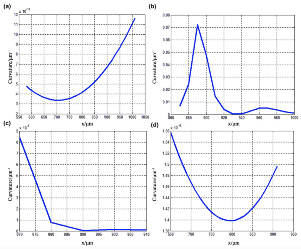
Fig. 23 Graphs of the curvature variations of the fitted curve for the characteristic curves (a) 1, (b) 2, (c) 3, and (d) 4 (Li et al., 2022).

Using these graphs, a connection between the geometrical structure and the function of that claw segment can be established.

In regards to the first claw segment, we can analyze the corresponding second derivative graph and curvature variation graph, both given by the graphs (a) in Figure 22 and Figure 23. The graph of the second derivative is negative, indicated by its concave shape, with its decreasing curvature. The graph of the curvature variation includes a slight change with a minimum value of less than 12×10-18µm^-1. This indicates a large curvature radius, a smooth contour surface, and gradual changes. Altogether, these geometric features of this claw segment provide reduced frictional resistance. Exploring relations between structure and function, this morphology can prevent this segment of the claw from adhering to bamboo shoots (Li et al., 2022).

Regarding the second claw segment, the corresponding second derivative graph and curvature variation graph were analyzed, both given by the graphs (b) in Figure 22 and Figure 23. The graph of the second derivative is positive, indicated by its convex shape. The graph of the curvature variation includes a sharp change with the most extreme value (indicating this segment of the claw contains the most severe curvature) with a maximum value between 0.07-0.08 µm^-1. This indicates a small curvature radius and a large degree of curvature. This graphical analysis indicates the pronounced arc shape of this claw segment, which punctures the bamboo shoots for improved grasp (Li et al., 2022).

As for the third claw segment, the corresponding second derivative graph and curvature variation graph were analyzed yielding the graphs (c) in Figure 22 and Figure 23. The graph of the second derivative is positive, indicated by its convex shape. The graph of the curvature variation includes bare changes without any noticeable extreme values. Overall, there is a decreasing curvature and increasing radius of curvature. Since this segment of the claw lacks relative curvature, adhesion forces are necessarily present here to aid in the claw's gripping abilities (Li et al., 2022).

In regards to the fourth claw segment, the corresponding second derivative graph and curvature variation graph can be analyzed, both given by the graphs (d) in Figure 22 and Figure 23. The graph of the second derivative is negative, indicated by its concave shape. The graph of the curvature variation includes a slight change with a minimum value of less than 1.56×10-18µm^-1. This indicates a large curvature radius, which continues to increase rapidly. This curvature enhances adhesion forces found in the previous claw segment by reducing stress concentration to improve structural strength and functionality of the claw itself (Li et al., 2022).

Overall, the geometry of the claw of Cyrtotrachelus buqueti Guer follows a contour curve moving from convex to concave to convex  when traced from the exterior to the interior of the claw. Following the same trace, the curvature changes from slightly curved to strongly curved (at the arc point) to slightly curved. As delineated, this curvature pattern enhances the claw's ability to utilize adhesion forces. Therefore, this geometrical structure ultimately improves the overall capabilities of the claw (Li et al., 2022).

With this data on the structure-function relationships between the geometry and the purpose of the claw of the Cyrtotrachelus buqueti Guer, there are many biomimetic applications that engineers can pursue, such as machines able to ascend vertical structures. Using mathematical models based on animal appendages, engineers can design devices that follow the intrinsic mathematical properties of nature for the most functionally effective instruments.

Mathematical modeling of vole claws

Evidently, nature yields the most effective tools for any required task. Over time, animals develop evolutionary adaptations that offer advantages in performing their essential daily tasks. For voles, also known as meadow mice, of which a specimen is shown in Figure 24, evolution has honed their claws to have especially curved shapes with a geometric structure optimized for efficiently tilling the earth. These adaptations enable voles to burrow better and traverse the subterranean, allowing them to more efficiently find the plants of their diet. Of course, these plants are often grown by farmers, who view voles as bothersome pests (Brittingham, 2007). Nevertheless, the ability of voles to move so effectively through the use of their streamlined claws provokes an analysis of the geometry that optimizes their claws for their functionality.

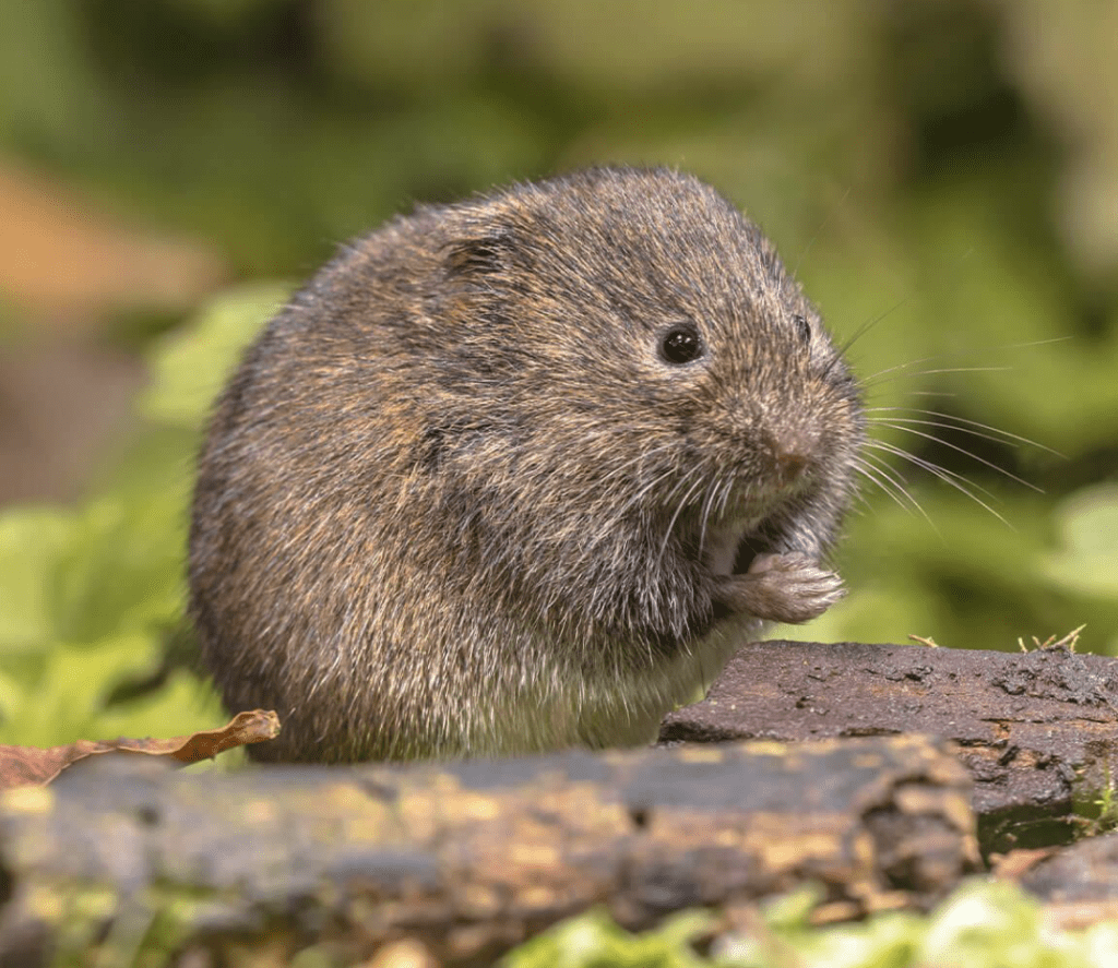
Fig. 24 Vole, otherwise known as a meadow mouse (Premier Tech Ltd., 2022).

In a study conducted by the Henan University of Science and Technology, researchers analyzed the claws of nine different digits of a vole (Guo et al., 2018). An image of each claw was amplified and placed on a Cartesian coordinate system – the inner proximal point of the claw was placed at the origin with the distal point on the claw extending into the fourth quadrant of the coordinate system, shown in Figure 25. These placements facilitated the comparison of the different claws for more in-depth mathematical analysis (Guo et al., 2018).

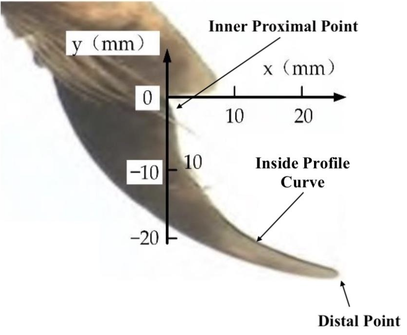
Fig. 25 Vole claw placed on a Cartesian coordinate system to facilitate observation and comparison between different claws analyzed (Adapted from Qui et al., 2022).

To generate a mathematical model of the inside profile curves of the claws, the researchers used the least squares method to fit the data points of the inside profile curves. Through several experiments, the researchers verified that the fourth-order polynomial function possessed the highest fitting precision compared to other functions tested. The fourth-order polynomial function used is given by Equation 9. The values of each of the coefficients along with the R² values for each of the nine claws' inside profile curves are shown in Table 3. Considering that high fitting precision is indicated by values of R² close to 1, the fourth-order polynomial function was accepted, yielding R² values within 0.01 units from 1 for each of the claws of the vole, indeed the function with the highest fitting precision (Guo et al., 2018).

f(x)=a_4x^4+a_3x^3+a_2x^2+a_1x+a_0

Eq. 9 Equation for fourth order polynomial function

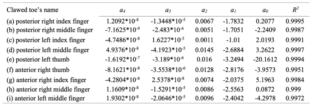
Table 3 Fourth-order polynomial function coefficients and R² values for each of the claws of the vole (Guo et al., 2018).

From the values from Table 3 used along with the fourth-order polynomial function given by Equation 9, the researchers constructed a graph by plotting the position coordinates to generate the fitting curves of the inside profile curves of the claws, as shown in Figure 26 (Guo et al., 2018).

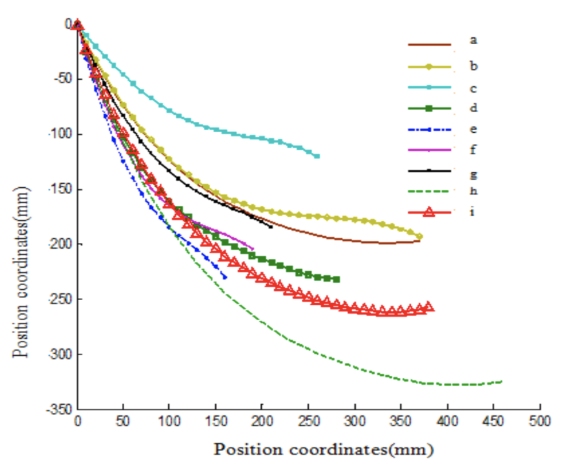
Fig. 26 Fitting curves of the inside profile curves of the claws (Guo et al., 2018).

Using these fitting curves and the unique fourth-order polynomial function for each, the researchers were then able to calculate the curvature of each point on the curve and generate the curvature trendlines of the inside profile curves of the claws. This is all compiled in a graph shown in Figure 27 (Guo et al., 2018).

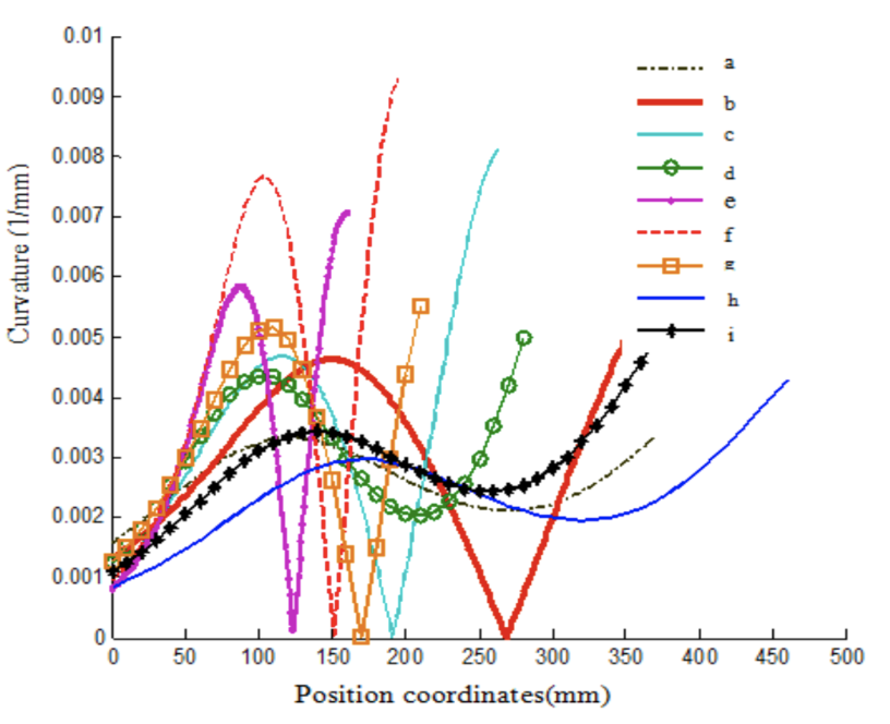
Fig. 27 Curvature trendlines of the inside profile curves of the claws (Guo et al., 2018).

As observed in Figure 27, the curvature trendlines experience several fluctuations. Corresponding to the proximal point of the claw, the curvature trendlines originate at a minimum. From there, the curvature trendlines gradually increase to a maximum that corresponds to the “center” of the inside profile curve. From there, the curvature trendlines gradually decrease to reach another minimum corresponding to the claw's distal point. From there, the curvature trendlines gradually increase to reach another maximum which corresponds to the ‘center' of the outside profile curve (not relevant in this discussion). Here the graph ceases as the rest of the claw structure is not relevant to this discussion. Overall, the graph of the curvature trendlines of the inside profile curves features two minimum points and two maximum points. For a more in-depth analysis of the geometric features of the inside profile curves of the claws, the researchers analyzed a generalized curvature trendline, as shown in Figure 28, and assigned each of the extreme points of the curvature trendline as points A, B, C, and D corresponding to the first minimum, first maximum, second minimum, and second maximum, respectively. Furthermore, the researchers defined the abscissas of the extreme points A, B, C, and D as X_a, X_b, X_c, and X_d, respectively (Guo et al., 2018).

Fig. 28 Generalized curvature trendline used to analyze the geometric features of the inside profile curves of the claws (Adapted from Guo et al., 2018).

From the abscissas, the researchers calculated the abscissa ratios from point B and point C to point D (point A is disregarded, considering its abscissa is X_a=0 mm due to the point's location on the y-axis), defined by X_b/X_d and X_c/X_d, respectively. With this data, the researchers were able to obtain the statistical eigenvalues of each datum, shown in Table 4 (Guo et al., 2018).

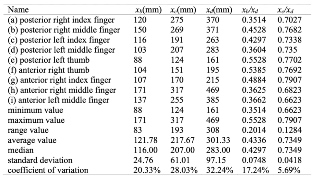
Table 4 Statistical eigenvalues of the abscissa of the extreme points (Guo et al., 2018).

From the data in Table 4, the coefficient of variation of X_b/X_d is less than the coefficient of variation of X_c/X_d for each of the claws. This designates X_c/X_d as less discrete than X_b/X_d. Nevertheless, both coefficients of variation for the abscissa ratios are small values, which indicates that the relative positions of the extreme points B and C are rather concentrated. This aligns with the data of the abscissa of the extreme points B and C considering X_b and X_c are relatively concentrated as well (Guo et al., 2018).

Moreover, the researchers defined the curvature values of the extreme points A, B, C, and D as K_a, K_b, K_c, and K_d, respectively. Calculating these values, the researchers obtained the statistical eigenvalues of the extreme points, shown in Table 5 (Guo et al., 2018).

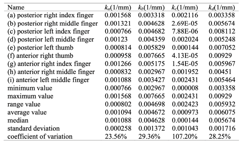
Table 5 Statistical eigenvalues of the curvature of the extreme points (Adapted from Guo et al., 2018).

From the data in Table 5, coefficients of variation for the curvature values of the extreme points, ordered from smallest to largest, were as follows: K_a, K_d, K_b, then K_c. The coefficients of variation for the curvature values of the extreme points A, D, and B are relatively concentrated. In contrast, the coefficient of variation for the curvature value of the extreme point C is more scattered. This aligns with the actual observable shape of the claw, considering point C corresponds to the distal point of the claw, which bears the least resemblance to the shape of the claw at the other points A, D, and B (Guo et al., 2018).

Overall, the characteristics of the variable curvature of the inside profile curves of the claws of the vole enable the animal to efficiently burrow and expeditiously traverse the subterranean due to the geometric structure of the claws effectively reducing resistance and providing anti-adhesion against the earth. Engineers can model tools, such as agriculture, after the claws of voles and other terrestrial animals by applying the geometrical curvature shape favored by nature and evolution in bionic optimization.

Mathematics of claws in amniotes

Four-legged vertebrates, or amniotes, such as reptiles and mammals, have claws. Although the power law explains the growth and shape of appendages such as claws, there are other ways to describe the pointed curve shape of the claw that supplements the power law. This can be used to do biomimicry of claws to model and produce tools to dig.

Claw shape in amniotes

The first model of the claw in amniotes, like the power law, uses a logarithmic spiral. This follows the constant stress hypothesis, where the parts with more stress are thicker, and those with less stress have less material (Matheck, 1991). Therefore, using arcs to describe a claw's properties is not ideal or precise. One property can be the von Mises stress represented as isolines on claws. The von Mises stress was originally used to measure the capacity of steel to not fracture, but it can also be used in a biological context (Matheck, 1991). There would be a stress peak at the tip of the claw, represented by the proximity of the lines, as seen in Figure 29. This stress would be lessened by using a logarithmic spiral for isolines. In nature, the claws would follow the second pattern (Matheck, 1991). However, using angles or pseudo landmarks to represent the shape of the claw can further the understanding of differences between claws of species.

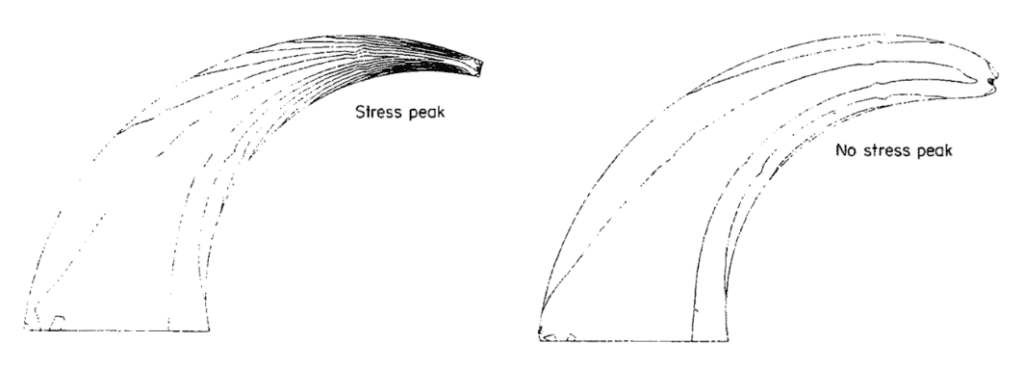
Fig. 29 A claw with arcs for isolines presenting a stress peak (left). and logarithmic isolines (right) (Adapted from Matheck, 1991).

The first alternative way to describe the shape of a claw in two dimensions is by measuring the underlying angle. The profile of a claw is curved and can be described by an upper and lower arc. The points considered are the beginning and end of the respective arc and the point of inflection if it is present (Tinius, 2016). A point of inflection is when a slope switches the direction of curvature. This point can usually be found by taking the second derivative of a function in mathematics. Visually, a point of inflection is described as the point where the curve changes from being concave up. The inflection point also goes from concave down to up. For curves that do not have an inflection point, the third point is taken from the intersection of the curve and the perpendicular line passing through the center between the end and beginning of the arc. Therefore, the angle that is taken into consideration is the one at the top of the triangle, touching the inflection point or the arc, as seen in Figure 30.

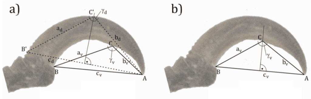
Fig. 30 Claw, of Picoides villosus, angle measured with inflection point as reference point at (a). Claw angle measured with the center of the triangle as reference point at (b) (Adapted from Tinius, 2016).

In the same animal, claws differ in terms of position and use. Back claws may require greater sturdiness to move, and the front may need more pointiness to catch prey. Species that stay on the ground have a smaller ratio between the hind claws compared to the fore claws (Baeckens, 2019). This deviates from climbing animals and those that live in heavy vegetation, which need sturdier back claws.

Another way to describe the shape of claws is by using geometric morphometric analysis. Every image of a biological part is marked with a given number of dots equidistant from one another (Tinius, 2016). Then the median of each dot position from a dataset, or specific animal, is computed and compared with other animals (Tinius, 2016). For the case of claws, 30 landmarks are used for each arc of the claw for a total of 60 landmarks, as seen in Figure 31.

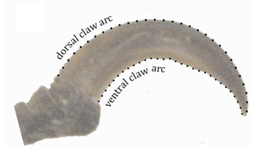
Fig. 31 An example of the placement of landmarks on the claw (Adapted from Tinius, 2016).

The number of points representing the claw shape is important as a large number would make the image very prone to inconsistencies due to irregularities in each specimen's claws. The simplistic nature of triangles and arcs does not hold back this technique to represent claws. Compared to measuring claw angles, this method considers more information such as the thickness of the claw profile (Tinius, 2016). However, as stated earlier, the increased precision may capture unwanted features such as the wear of the claw tip.

Morphometric analysis can also be used to identify real claws from fake claws. Morphometric analysis englobes many tests, such as burning the material or taking measurements (Vipin, 2016). In the black-market trade of claws, the merchandise seized is sometimes made up of fakes and investigators must know how many are real to see the extent of the trade. For this purpose, visual inspection is often insufficient. The measurements taken for analysis are the distance between the tip and the beginning of the lower arc and the distance between the upper and lower base of the claw, as seen in Figure 32.

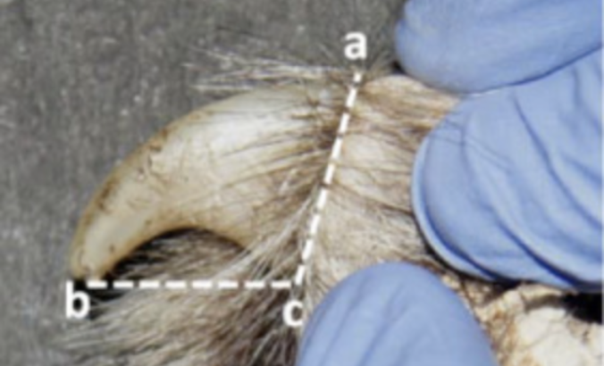
Fig. 32 The lines of both measurements taken from the claws to determine the ratio of claw base and length of claw (Adapted from Vipin, 2016).

These two measurements are put in a ratio that can be compared with a sample ratio from real tiger or leopard claws, as seen in Table 6. Even if the claws have the right dimensions, they may still be replicas. Out of 18 seized claws in a study, four had the correct dimensions, but were still found to be fake (Vipin, 2016).

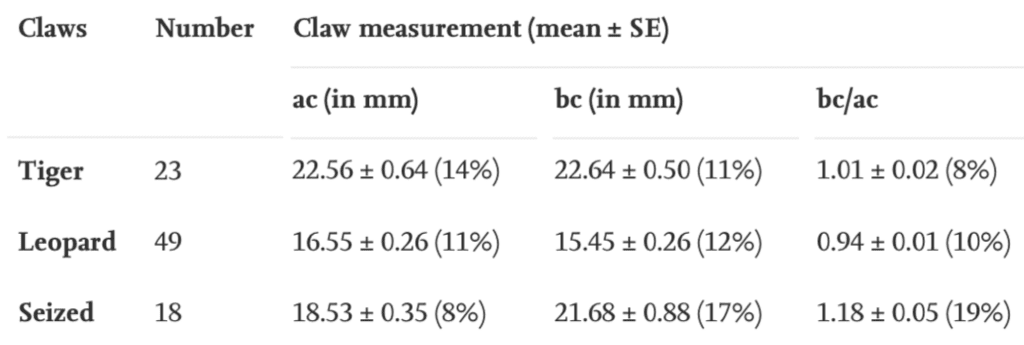
Table 6 Measurements taken from the claws of tigers and leopards compared to seized claws (Adapted from Vipin, 2016).

Further testing is done using an x-ray to identify the density of the keratin in the claw. Fake claws do not have a gradient density of keratin, meaning that the keratin does not become less dense at the edges (Vipin, 2016). The use of measurements before x-rays or PCR tests hastens the process of identifying the claws as other techniques can be time consuming or resource intensive. The better fakes can be made of cattle keratin, allowing the fake claws to slip past the initial tests meant to identify the materials of the seized claws (Vipin, 2016). To increase the scope of the morphometric analysis for claws, more animals must be added to the database so the measured claw ratio can be compared to more animals. By having a wider range of samples, the people that seize the claws could identify whether the claw belonged to an animal faster at a lesser cost.

The use of bionic claws for digging or soil loosening

The many ways to describe claws can be helpful in biomimicry, allowing for the creation of technologies that can benefit or improve existing techniques. One of the many uses of claws is digging, and an example of a rudimentary tool that resembles a claw is a hoe. This tool consists of a handle and a pointed piece intended to loosen dirt. By describing the claws mathematically, the software can model the shape of claws and simulate different conditions on designs of bionic claws in the development of hoe technology (Guo, 2009). 

The goal is to increase the efficiency of the bionic claw that moves in the substrate and lessen the friction created by the movement of the piece (Guo, 2009). A simple way to quantify these characteristics is to make claws with various longitudinal dept ratios, then measure the amount of soil displacement, as seen in Figure 33. The depth refers to how deep the claw is put into the soil when loosening it. The slope of the inner portion of the claw has a curvature that changes throughout the claw (Guo, 2009).

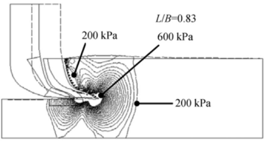
Fig. 33 Model of a bionic claw and soil displacement. L is the longitudinal distance between the base of the claw and the tip, B is the depth, and L/B is the longitudinal depth ratio (Adapted from Guo, 2009).

After modeling several lengths, the researchers found that the ideal longitudinal depth ratio is 0.8 (Guo, 2009). This means that the depth of the claw should be larger than the longitudinal distance between the base and the tip of the claw. This ratio reduces the resistance of the soil and, along with the change in curvature, reduces friction and breaks the soil more efficiently (Guo, 2009).

An animal that is good at plowing and digging is the brown bear. The brown bear's claws experience little resistance in the dirt due to their shape (Sun et al., 2020). By modeling the claws digitally, as seen in Figure 34, and printing them, one can make a ditching blade holder with the claws at the tips (Sun et al., 2020). A ditching blade is the part of the plowing machine that loosens up the dirt, as seen in Figure 34.

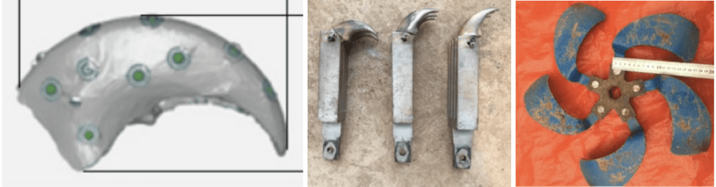
Fig. 34 A bear claw modeled in software on the left, bionic claws in the middle, and a ditching blade on the right (Adapted from Sun et al., 2020).

Many sizes and angles of claws are used to find the most efficient combination, as seen in Figure 34. Compared to the average ditching blade available on the market, the bionic claw requires less energy to produce the same amount of displacement (Sun et al., 2020). For the same rotation speed and depth, the ditching blade consumed 249 kJ/m³, while the bionic claws consumed 236 (Sun et al., 2020). A reduction in energy is important as there is a lot of soil to move. As such, there would be a reduction in costs if more ditching blades were made of bionic claws (Guo, 2009). More tests would be necessary to see if the manufacturing and maintenance of these bionic claws is still advantageous compared to the normal blades.

Conclusion

The many mathematical approaches to analyzing the claw reveals how it has been optimized by evolution for its many purposes. Whether foraging, hunting, climbing, or digging, an animal's claws are impeccably suited for their specific function. The logarithmic spiral, responsible for forming claw curvature, and the power cascade, which forms the claw's volume, describe the claw growth that allows for the balance of stress placed upon the claw while still creating a tool capable of serving diverse mechanical demands. This mathematically constrained growth enables scientists to draw patterns between claw curvature and ecological niche to make predictions about extinct species, such as the Archaeopteryx, and learn about the evolution of capabilities such as flight. Furthermore, conclusions can also be drawn on the size of prey relative to claw size of predatorial raptors due to strong correlation between the two, demonstrating the specialization potential of claw growth to best suit the animal. This pattern is reinforced when examining the claw of the Cyrtotrachelus buqueti Guer, which demonstrates a contour curve that alternates between convex, to concave, to convex, showing remarkable complexity in its growth to best achieve adhesive capability and claw strength. The claws of the vole also can be characterized by variable curvature inside the profile curves, which optimizes for reduced resistance during digging and anti-adhesion against soil. These many capabilities can be mimicked into human tools through geometric morphometric analysis and angular analysis in order to harness solutions developed by many millennia of evolution – for example, bionic claws can be made to mimic the digging properties of brown bear claws, opening the door for many more biomimetic technologies to develop. In this way,  it can be seen how the mathematical analysis of claws may prove greatly beneficial to the development of biomimetic technology, as well as its use in modeling and paleontology.

References

Alibardi, L. (2016). The Process of Cornification Evolved from the Initial Keratinization in the Epidermis and Epidermal Derivatives of Vertebrates: A New Synthesis and the Case of Sauropsids. International Review of Cell and Molecular Biology, 327, 263–319. https://doi.org/10.1016/bs.ircmb.2016.06.005

Baeckens, S., Goeyers, C., & Van Damme, R. (2019). Convergent Evolution of Claw Shape in a Transcontinental Lizard Radiation. Integrative and Comparative Biology, 60: 10-23. https://doi.org/10.1093/icb/icz151

Birn-Jeffery, A. V., Miller, C. E., Naish, D., Rayfield, E. J., & Hone, D. W. E. (2012). Pedal Claw Curvature in Birds, Lizards and Mesozoic Dinosaurs – Complicated Categories and Compensating for Mass-Specific and Phylogenetic Control. PLoS ONE, 7(12), e50555. https://doi.org/10.1371/journal.pone.0050555

Bouchner, M. (1977). Birds of Prey of Britain and Europe. London: Hamlyn Publishers.

Britannica, T. Editors of Encyclopaedia (2022, September 23). spiral. Encyclopedia Britannica. https://www.britannica.com/science/spiral-mathematics

Brittingham, M. C. (2007, January 5). Voles. Penn State Extension | The Pennsylvania State University. https://extension.psu.edu/voles

Cade, T. J. (1982). The Falcons of the World. Comstock/Cornell University Press.

Cook, J. D. (2022, May 9). Logarithmic spiral. In John D. Cook Consulting. https://www.johndcook.com/blog/2022/05/09/logarithmic-spiral/

Csermely, D., & Rossi, O. (2006). Bird claws and bird of prey talons: Where is the difference? Italian Journal of Zoology, 73(1), 43–53. https://doi.org/10.1080/11250000500502368

Evans, A. R.; Pollock, T. I.; Cleuren, S. G.; Parker, W. M.; Richards, H. L.; Garland, K. L.; Fitzgerald, E. M.; Wilson, T. E.; Hocking, D. P.; Adams, J. W. (2021) A Universal Power Law for Modelling the Growth and Form of Teeth, Claws, Horns, Thorns, Beaks, and Shells. BMC Biology, 19 (1). https://doi.org/10.1186/s12915-021-00990-w 

Feduccia, A. (1993). Evidence from Claw Geometry Indicating Arboreal Habits of Archaeopteryx. https://doi.org/10.1126/science.259.5096.790

Feldhamer, G. A.; Merritt, J. F.; Krajewski, C.; Rachlow, J. L.; Stewart, K. M. Mammalogy: Adaptation, diversity, ecology; Johns Hopkins University Press: Baltimore, Maryland, 2004.

Fowler, D. W., Freedman, E. A., & Scannella, J. B. (2009). Predatory Functional Morphology in Raptors: Interdigital Variation in Talon Size Is Related to Prey Restraint and Immobilisation Technique. PLoS ONE, 4(11), e7999. https://doi.org/10.1371/journal.pone.0007999

Glen, C. L., & Bennett, M. B. (2007). Foraging modes of Mesozoic birds and non-avian theropods. Current Biology, 17(21), R911–R912. https://doi.org/10.1016/j.cub.2007.09.026

Guo, Z., Jia, D., Deng, L., & Chen, Y. (2018). Statistical law of variable curvature characteristics on the inside profile of the vole's clawed toes. IOP Conference Series: Materials Science and Engineering, 382, 052023. https://doi.org/10.1088/1757-899x/382/5/052023

Guo, Z., Zhou, Z., Zhang Y., & Li, Z. (2009). Bionic optimization research of soil cultivating component design. Science in China Series E: Technological Sciences, 52: 955-965. https://doi.org/10.1007/s11431-008-0208-4

Hedrick, B. P., Cordero, S. A., Zanno, L. E., Noto, C., & Dodson, P. (2019). Quantifying shape and ecology in avian pedal claws: The relationship between the bony core and keratinous sheath. Ecology and Evolution, 9(20), 11545–11556. https://doi.org/10.1002/ece3.5507

Horstman, J. (2013, August 24). Giant Bamboo Weevil (Cyrtotrachelus buqueti, Curculionidae) [Photograph]. Flickr. https://www.flickr.com/photos/itchydogimages/10282795854

Horstman, J. (2013, August 24). Giant Bamboo Weevil (Cyrtotrachelus buqueti, Curculionidae) [Photograph]. Flickr. https://www.flickr.com/photos/itchydogimages/9609675145/in/photostream/

Kang, S. H., & Kim, J. Y. (2021). Application of Fast Non-Local Means Algorithm for Noise Reduction Using Separable Color Channels in Light Microscopy Images. International Journal of Environmental Research and Public Health, 18(6), 2903. https://doi.org/10.3390/ijerph18062903

Li, L., Sun, W., Guo, C., Guo, H., Lili, L., & Yu, P. (2022). Mathematical model and nanoindentation properties of the claws of Cyrtotrachelus buqueti Guer (Coleoptera: Curculionidae). IET Nanobiotechnology, 16(6), 211-224. https://doi.org/10.1049/nbt2.12089

Lyon, R. D. (2011, February 1) Logarithm. In Wikipedia. https://en.wikipedia.org/wiki/Logarithm#/media/File:Logarithm_plots.png

Matheck, C., & Reuss, S. (1991) The Claw of the Tiger: An Assessment of its Mechanical Shape Optimization. J. theor. Biol., 150: 323-328. https://doi.org/10.1016/S0022-5193(05)80431-X

Neuman, S. (2014, November 13). Barn Owl. Audubon. https://www.audubon.org/field-guide/bird/barn-owl

Premier Tech Ltd. (2022). Voles. Wilson insect, weed and rodent controls | Wilson Control. https://www.wilsoncontrol.com/rodent-control/glossary/voles

Qiu, Y., Guo, Z., Jin, X., Zhang, P., Si, S., & Guo, F. (2022). Calibration and verification test of Cinnamon soil simulation parameters based on discrete element method. Agriculture, 12(8), 1082. https://doi.org/10.3390/agriculture12081082

Raab, H. (2022). Archaeopteryx. In Wikipedia. https://en.wikipedia.org/w/index.php?title=Archaeopteryx&oldid=1121082471

Sun, J., Chen, H., Wang, Z., Ou, Z., Yang, Z., Liu, Z., & Duan, J. (2020). Study on plowing performance of EDEM low-resistance animal bionic device based on red soil. Soil and Tillage Research, 196. https://doi.org/10.1016/j.still.2019.104336

Tinius, A., & Russell A. P. (2016). Points on the curve: An analysis of methods for assessing the shape of vertebrate claws. Journal of Morphology, 278: 150-169. https://doi-org.proxy3.library.mcgill.ca/10.1002/jmor.20625

Tsang, L. R., Wilson, L. A. B., Ledogar, J., Wroe, S., Attard, M., & Sansalone, G. (2019). Raptor talon shape and biomechanical performance are controlled by relative prey size but not by allometry. Scientific Reports, 9, 7076. https://doi.org/10.1038/s41598-019-43654-0

Vipin, V. S., Sharma, C. P., Kumar, V. P., & Goyal, S. P. (2016). Pioneer identification of fake tiger claws using morphometric and DNA based analysis in wildlife forensics in India. Forensic Science International, 266: 266-233. https://doi.org/10.1016/j.forsciint.2016.05.024

Yang, H., Su, T., Yang, W., Yang, C., Lu, L., & Chen, Z. (2017). The developmental transcriptome of the bamboo snout beetle Cyrtotrachelus buqueti and insights into candidate pheromone-binding proteins. PLOS ONE, 12(6), e0179807. https://doi.org/10.1371/journal.pone.0179807