Copepods Through the Lens of Math

Johanna Turton, Melodi Rousset, Philippe Mercier, Tanjin Sultana

Abstract

The silent artistic order of the natural world has been revealed through mathematical concepts such as the Fibonacci sequence or the Golden Ratio. The beauty of nature is not random chaos but a manifestation of seemingly abstract mathematics. This review paper will present copepods through the distinct lens of mathematics. As these fascinating creatures continue to captivate researchers across various disciplines, this paper delves specifically into the mathematical models developed to understand their unique attributes. Furthermore, topics such as copepod clustering and growth and development kinematics will be introduced and explored through mathematics. This paper will demonstrate that, despite their tiny size, copepods are a fascinating example of the relationship between nature and mathematics. By exploring this relationship, we can gain a better understanding and admiration of both.

Introduction

Copepods are perplexing creatures found in almost every body of water around the world. They make up a diverse and ecologically significant group within the zooplankton community. The study of copepods can be complicated due to their nature and environment. Therefore, the math of copepods can serve as a lens to provide further insight into the physiology, physics, and chemistry of these adaptations. Mathematical models are an important tool that will be used in this paper to bridge the gap between empirical observations and theoretical models. These models will demonstrate the calculation-based and exact nature of copepod's unique design solutions. Moreover, these models will show that these mechanisms are not lucky guesses, but precise solutions designed and perfected by nature through millions of years of evolution.

Copepods face the challenge of navigating through environments characterized by low Reynolds numbers, where viscous forces dominate inertial forces. In this paper, we explore mathematical models that capture the distinctive propulsion mechanisms employed by copepods. These models offer insights into the behaviors of copepod swimming, shedding light on the strategies copepods employ to efficiently move and forage. The kinematics of the growth of copepods will demonstrate the key factors governing their development. This paper will explore the interesting molting rule and its role in reproduction and body size which lays the foundation for understanding the different stages of life of a copepod. Not to mention, this paper explores Lagrangian models to elucidate the clustering of copepods. Additionally, we delve into the intriguing phenomenon of copepod color adaptation, specifically focusing on the role of guanine plates in altering their coloration. The mathematical perspective of this process is examined through matrix calculations, offering a quantitative approach to understanding how copepods dynamically adjust their coloration in response to their environment. As mathematical models unveil the mysteries of copepods, this review paper will dive into the mathematics that govern their unique yet wonderful behaviors.

Copepods' displacement at low Reynolds numbers

Context

In a previous work, it was explained how living at low Reynolds numbers poses challenges to copepods when it comes to feeding through the lens of physics. As a reminder, the Reynolds number of a system represents the ratio of inertial forces over viscous forces acting on a body. Copepods living at low Reynolds numbers thus means that their world is dominated by viscous forces such that they cannot rely on momentum to accomplish daily tasks like catching food particles and bringing them to their mouths.

In this section, the focus will rather be made on how copepods manage to overcome the challenges that low Reynolds numbers pose in terms of displacement and thereby, in terms of escaping predators. In fact, at high Reynolds numbers (10⁶, for example, which is the Reynolds number for humans in water), displacement in fluid can be achieved by performing a symmetric and synchronous movement fast with two limbs, and then making the reciprocal of that movement more slowly. This is because the propulsion brought by the first movement causes the accumulation of enough inertia for the object to travel significantly through space against the viscous forces, which are weak enough for the reciprocal movement not to, when made slowly, propel the body back into its original emplacement (Purcell, 1977). At the low Reynolds numbers however (10^-1 for example, the Reynolds number of copepods in water), the inertial forces are so negligible compared to the viscous forces that such a combination of a synchronous, symmetric movement and its reciprocal would result in no net displacement (Purcell, 1977).

Because of that, copepods have evolved a different way of swimming, which consists of moving their legs simultaneously during a propulsive stroke, then moving them asynchronously during the recovery stroke (Shanbrom et al., 2021). Below, this low Reynolds number adapted method of swimming will be analyzed via a mathematical model, which will allow for a better understanding of how such a swimming technique succeeds where high Reynolds numbers' ones fail.

Mathematical model

In general, the state of a copepod having “n” legs can be modeled as follow (Shanbrom et al., 2021):

$\dot{q}(t) = \sum_{i=1}^{n} \dot{\theta}_i(t) F_i(q(t)) \quad (1)$

Here, “q(t)” corresponds to (x(t), y(t), φ(t))^T and represents the state of the copepod in a two-dimension plane – its position according to the x and y-axis, and its orientation “φ” according to the x-axis. Hence, “ $\dot{q}(t)$ ” represents the motion of the body of the copepod – its change in state – as a function of the angular velocity of its legs “ $\dot{\theta}$ ” and the parameter “F”, which is such that

$F_i = M_i^{-1} K_i \quad (2)$

where “M_i” is the matrix describing the resistance to leg movement caused by the fluid viscosity, “M_i^-1”, the mobility matrix, and “K_i”, the actual rotative motion of the i^thleg according to the x axis. At copepods' Reynolds number, where the inertia can be neglected, the Navier-stokes equations lead to the following functions for “M_i” and “K_i” (Shanbrom et al., 2021):

$M_i = \begin{bmatrix}1 + \sin^2(\alpha_i) & -\sin(\alpha) \cos(\alpha_i) & -\sin(\alpha_i) \\-\sin(\alpha) \cos(\alpha_i) & 1 + \cos^2(\alpha_i) & \cos(\alpha_i) \\-\sin(\alpha_i) & \cos(\alpha_i) & 2\end{bmatrix} \qquad (3)$

$K_i = \begin{bmatrix}\sin(\alpha_i) \\-\cos(\alpha_i) \\-\frac{3}{2}\end{bmatrix} \quad (4)$

Here, “ $\alpha_i$ ” is the angle between the i^th leg and the x-axis, while “ $\theta_i$ ” is the angle between the i^th leg and the orientation of the copepod – see Figure 1.

Figure 1: Hypothetical copepod with two legs – n=2 – the legs being the yellow line and the purple line (Shanbrom et al., 2021)

This model thus allows to know the effect of moving “n” legs at the same time on the velocity of the copepod in the x and y axis, as well as on its angular velocity – its change in orientation.

Hence, integrating the different components of $\dot{q}(t)$ results in calculating the overall change in position and orientation of the copepod following this given leg movement (Shanbrom et al., 2021). This is what will be used in the next section.

Use of the mathematical model to understand the swimming behaviour of the copepods

By solving the equation (1) with n = 2 explicitly for the change in orientation of the copepods with time and integrating this equation for the total orientation change – and doing the same for the position of the copepod over time – it is possible to calculate the overall change in orientation and position undergone by a hypothetical two legged copepod moving its legs according to the following pattern (Shanbrom et al., 2021):

$\theta_1(t) =\begin{cases}t & 0 \leq t < \pi \-2t + 3\pi & \pi \leq t < \frac{3\pi}{2} \0 & \frac{3\pi}{2} \leq t < 2\pi\end{cases}$ ,

$\theta_2(t) =\begin{cases}t + \pi & 0 \leq t < \pi \2\pi & \pi \leq t < \frac{3\pi}{2} \-2t + 5\pi & \frac{3\pi}{2} \leq t < 2\pi\end{cases} \quad (5)$

This pattern corresponds to the simultaneous displacement of the two legs by an angle of radians in the counterclockwise direction, followed by the reciprocal movement being made by both legs one after the other – the same movement but in clockwise direction.

Considering that the initial state of the copepods was

$q(0)=(x(0), y(0), \phi (0), \theta_{1}(0), \theta_{2}(0))^{T} = (0,0,0,0,\pi)^{T} \qquad (6)$

the final state of the copepods is calculated – following the above-mentioned procedure – as being:

$q(2\pi)=(x(2\pi), y(2\pi), \phi (2\pi), \theta_1(2\pi), \theta_{2}(2\pi))^{T}= (0.0071,0019,−\pi / 6,0,π)^{T} \qquad (7)$

There is thus a net displacement that occurs when the pattern (5) is made by the copepod, which comes from the fact that the propulsive part of the movement created more displacement than the recovery one (Shanbrom et al., 2021).

Mathematical model: conclusion

The fact that there is a net displacement when the pattern (5) is made by the copepod suggests that, at low Reynolds numbers, moving two adjacent legs at the same time creates more than twice the propulsion that moving one leg individually creates. This is how copepods can swim using reciprocal movements despite being in low Reynolds number environments by moving their legs synchronously during their propulsive strokes and asynchronously during the recovery strokes, an adaptation that has been helping them escape predators efficiently for millennia and become the most common group of animals on earth.

Diel vertical migration of copepods

Context

Every night, at dusk, copepods take part in the greatest daily migration on earth in terms of amount of biomass displaced: the diel vertical migration (Meester, 2010). This migration consists of copepods swimming 30-40 m upwards towards the surface at dusk – from a depth of around 35-45 meters to one of 1 to 5 meters – and swimming back down at dawn. This distance corresponds to more than 40 x 10³times the length of copepods. Scaled to humans, this would correspond to around… 60 miles! (Meester, 2010). At the surface, there is more food and more predators, hence, at night, when the latter are less efficient, it is beneficial for the copepods to inhabit the food-rich region of the ocean. During the day, however, it is beneficial for copepods –particularly the pigmented ones – to be as far away from the predator infested surface as possible (Meester, 2010). This migration also has some other benefits, and the following mathematical model highlights a specific one: it allows to maintain the copepods into the upwelling zone close to the seashore – see Figure 2 – which is the emplacement in the horizontal plane where food is most abundant for copepods (Wroblewski, 1982) (Peterson, 1998).

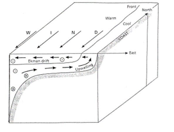
Figure 2: Upwelling happens most often in the zone close to the sea shore, and is due to wind blowing across the ocean and pushing the top layer water away, making the lower layer “upwell” to replace it (Peterson, 1998). Note that closer to the shore and the surface of water, food is more abundant for copepods.

Mathematical Model

For his simulation, J. S. Wroblewski modelized the population dynamics of the copepods species Calanus Marshallae as follows:

$\frac{\partial Z}{\partial t} + u \frac{\partial Z}{\partial x} + (w + w_s) \frac{\partial Z}{\partial z} - K_h \frac{\partial^2 Z}{\partial x^2} - K_v \frac{\partial^2 Z}{\partial z^2} = \text{population dynamics} \quad (8)$

where “Z” the population concentration per meter cubed, t is the time, x is the distance from the shore, z is the depth, K_h and K_vare coefficient assumed constant, u is the horizontal water velocity, w is the vertical water velocity, and w_sis the swimming velocity of copepods, which is equal to their maximum velocity multiplied by sin(2 $\pi t$ ), to account for their diel vertical migration pattern (Wroblewski, 1982).

This mathematical expression of the population dynamics of Calanus Marshallae in an upwelling region allowed to model the population emplacement in the x-z plane according to time as follows:

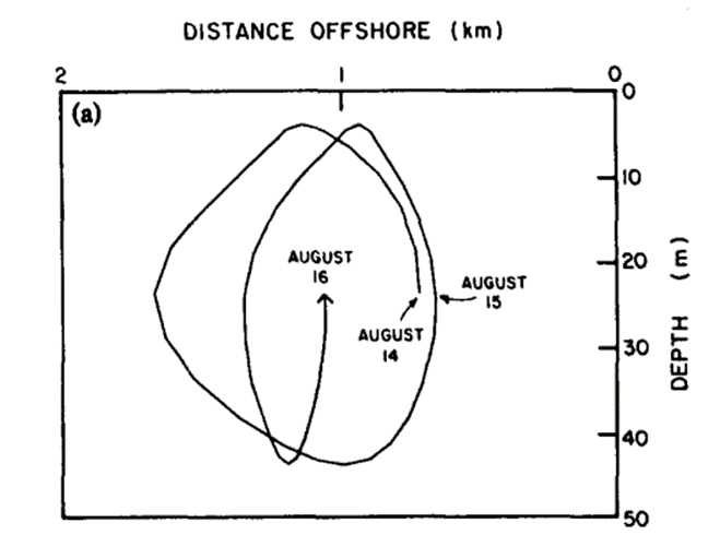
Figure 3: Circular motion described by Calanus Marshallae as they undergo diel vertical migration in an upwelling region (Wroblewski, 1982).

It can be seen in Figure 3 that the offshore displacement of the copepod population during the night due to their presence in the higher waters – which move offshore because of the Ekman drift, see Figure 2 – is compensated by their displacement onshore during the day, when they are deeper in the upwelling waters, hiding from predators (Wroblewski, 1982).

Conclusion from the mathematical model

This mathematical model allows to see how vertical migration allows copepods to remain into the nutritionally advantageous, close-to-the-shore upwelling region (Wroblewski, 1982). In other words, copepods have evolved a diel vertical migrating behavior as a solution to both the problem of having lots of diurnal predators where their food primarily is and the problem of being carried away from nutritionally favorable environments by water currents if always remaining in the food-rich, upper layer of water.

Copepod growth and development kinematics

Copepod development can be measured and modeled mathematically to better understand how they grow and reproduce. Many organisms reproduce based on reproduction cycles, seasons, or when the organisms reach a certain age. In copepods, research suggests they reproduce based on food supply (van den Bosch & Gabriel, 1994). Copepods grow through a process known as molting; during molting the copepod produces a new larger exoskeleton (also known as carapace) to replace that of the existing (Eichner et al., 2015). Copepods undergo molting several times within their lifespan depending on the species of copepod. There are three stages to copepod development, the nauplius stage, copepodite stages (also known as instar), and adult stage. The nauplius stage is the initial stage in which the copepod is hatched. The copepod then goes through multiple copepodite stages where copepod molts at each stage to grow. The adult stage is the final molt when at which time a copepod reaches maturity. At this point, the copepod can reproduce. The initiation and rate of molting are dependent on external factors such as food supply. The copepod will not undergo molting until the exoskeleton is complete. The synthesis of the exoskeleton is dependent on the investment of carbon in the building blocks of the carapace. The thickness of the exoskeleton is proportional to the length of the copepod, cubed. This is also proportional to the volume and weight of the copepod. Based on this observation van den Bosch & Gabriel were able to come up with a molting rule:

“Molt to the next instar when and if the net accumulated carbon allocated to carapace building bricks during the current instar reaches a fixed fraction of the body mass at the beginning of the current instar.” (van den Bosch & Gabriel, 1994)

Using this molting rule, they were able to create a model that calculates for each stage of growth the biomass of the copepod as well as feeding rate in relation to the size of the copepod. In order to understand the models that will be shown, we must understand the variables shown in Figure 4. From these variables we will be able to mathematically depict when the copepod will begin molting, length mass relations, and food intake relationship to growth.

Figure 4: variables associated with mathematical models of copepod growth (van den Bosch & Gabriel, 1994)

During the molting the carbon content of the carapace building bricks is a function (S_i(t)) where time is zero. The molt will begin if S_i(t), carbon content as a function of stage duration, is equal to the amount of carbon required to reach a certain length. These equations are shown in Formula 1. The first equation describes that when carbon concentration is proportionally equal to fraction of volume reserved to store carapace building bricks, the length-carbon content ratio, and the length of the copepod; the copepod will begin to undergo molting. The second equation states that during the stage, all carbon is allocated to molting and the concentration of carbon concentration of the carapace building brick storage is therefore zero.

molt if: $S_i(\tau_i) = \eta(\upsilon L_i^\sigma)$

at the molt $s_{i+1}(0) = 0$

Formula 1: concentration of carbon in relation to when the copepod will molt and during molting (van den Bosch & Gabriel, 1994)

Between molts copepods do not increase mass but they do however increase biomass. The equation in Formula 2 describes the ‘on-average' description of the relationship between weight and length. When the molt begins, the new length is determined by the current biomass of the copepod. Therefore, the total carbon content of the copepod at the end of a stage determines the length of the copepod at the next stage.

$\text{biomass} = \upsilon \cdot \text{length} \cdot \sigma$

Formula 2: describes the relationship between biomass and length of copepod with length-carbon ratios. (van den Bosch & Gabriel, 1994)

Feeding rates of copepods are heavily dependent on food density (x) and research has shown that copepod size increases with food density to an upper limit. Basically, the maximum amount of carbon that is able to be absorbed is proportional to food density in the environment as well as the size of copepod as shown in Formula 3. In the equation, ø usually varies between 0.79 and 1 with an average of 0.85. These values were obtained from looking at a variety of different food density papers completed by: Berggreen et al. (1988), Ambler (1986), Hamburger and Boetius (1987), Harris and Paffenhijfer (1976), Paffenhofer and Harris (1971), and Santer and van den Bosch (1994).

$F_i = I_m \frac{\alpha x}{1 + \alpha x} (\upsilon L_i^\sigma)^\theta$

Formula 3: shows the relationship between food intake and size of copepod along with food density. (van den Bosch & Gabriel, 1994)

The amount of food, i.e. carbon, the copepod intakes, influences not only the size of the copepod but how quickly it goes through the stages of development to the adult stage. This equation can be further analyzed by experimental data obtained in Figure 8. We can see from this figure that food density decreases the amount of time between stages (top graph), increases biomass (middle graph) and increases the length of copepod (bottom graph).

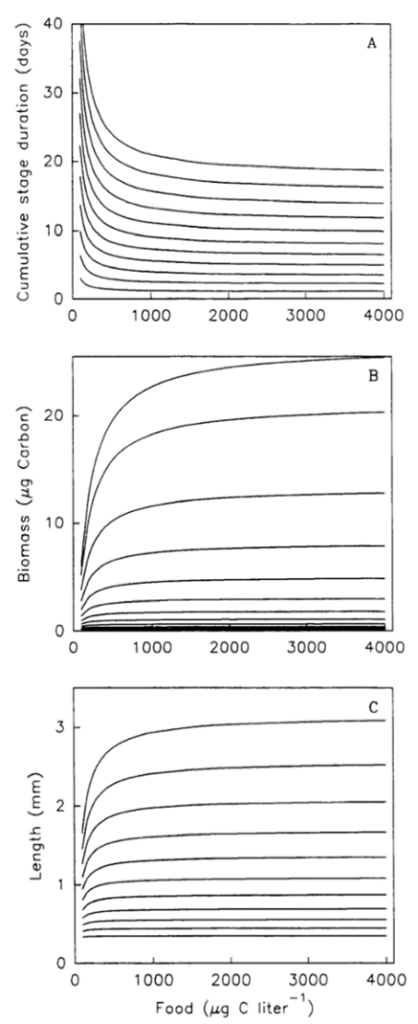
Figure 8: Impact of food density on time stage duration, biomass, and length of copepod. (van den Bosch & Gabriel, 1994)

Copepods do not begin to reproduce until they enter the adult stage. As we have shown from the equations and graphs, stage time as well as number of stages to reach desired size of copepod (biomass and length of copepod) are both dependent on food density. Therefore, rather than being dependent on the age of the copepod or the seasons, copepod reproduction is dependent on their development stages. Their development stages are in turn dependent on external factors such as food density. If copepods do not have an adequate food supply, they will not intake enough carbon and will not develop to a reproductive state. They need enough food (carbon) to not only stay alive, but to molt and develop into the reproductive adult stage.

Understanding why copepods cluster

Copepods are secondary producers thus they have a significant role in the marine ecosystem as they link phytoplankton cells (primary producers) to fish larvae or large mammals such as whales (Ardeshiri et al., 2016). For that reason, it is crucial to understand their dynamics within the ocean. As we approach the end of our story on copepods, we have already mentioned how copepods sense predators via hydrodynamical disturbances they sense through their antennae and how they capture their prey via generating feeding currents or ambush feeding (Paper 1: Physics). Within this section, we will explore more how they use behavioral methods such as clustering to provide many benefits especially to reduce the stress caused by turbulent flows (Ardeshiri et al., 2017).

Back in 2016, researchers Ardeshiri et al., were interested in knowing how copepods would interact within turbulent flows (Ardeshiri et al., 2016). This can be dependent on many factors such as the organism's size, morphology, its abundance, and most importantly hydrodynamic turbulence. It is known that when copepods are uncomfortable, they can escape, and copepod's velocity can reach 0.5 m/s while their mechanical energy can reach 8*10^-5 J/s which is why they are known to be the fastest and strongest animals in the world despite being so microscopic in size!

For that reason, they used the Lagrangian copepod model on active particles to depict how copepods move. This model is quite complex thus, before we dive into it, let us discuss the assumptions and the conjecture that the experimenters made:

List of Assumptions

The model ignores any swimming activity done by copepods that is related to finding food, or chemoreception.
Copepods always respond to disturbances via jumping.
Copepods do not modify the flow.
Copepod-copepod interactions are neglected.
Only the drag force is considered during the jumps.
Copepods are assumed to be spherical in shape.
The jump cannot begin until the previous jump is finished.
A jump is done when the amplitude of the copepod is negligible (i.e, 1% of the initial amplitude). The amplitude in this case refers to the height of the jump.

Conjecture

Copepods are small $\rightarrow$ Their centre of mass is represented as a fluid tracer $\rightarrow$ Helps with detection of flow patterns.

The most important assumption is that when the hydrodynamic disturbance generates a mechanical signal known as the strain rate, $\dot{\gamma}$ , copepods get triggered to escape. Once the strain rate reaches a threshold, $\dot{\gamma}_T$ , the copepod can initiate a jump. To understand the strain rate, the formula is denoted by:

$\dot{\gamma} = \sqrt{\sum_{i=1}^{1} \sum_{j=1}^{3} \frac{1}{2} \left( \partial_i u_j + \partial_j u_i \right)^2}$

where the $u_j$ and $u_i$ represent the fluid velocity field in three dimensions (i=1,2,3) and (j=1,2,3) and the components $\partial_i u_j$ and $\partial_j u_i$ represent the shear strain (refer to paper 1) and the normal strain respectively where shear strain dominates within turbulent flows (Ardeshiri et al., 2017).

The LC (Lagrangian-copepod) equation of a particle in motion can be denoted as:

$x(t) = u(x(t), t) + J(t, t_i, t_e, \dot{\gamma}, p)$ ,

where u(x(t), t) is the velocity of the carrying fluid at position x(t) at time t, and J describes velocity of the jump of the copepod where it's a function of time t, the initial and final time depicted by ti and te respectfully, the shear rate, and the orientation vector p.

The jump term could be expanded to this formula:

$J(t, t_i, t_e, \dot{\gamma}, p) = H[\dot{\gamma}(t_i) - \dot{\gamma}_T] H[t_e - t] u_J e^{\frac{t_i - t}{\tau_J}} p(t_i)$ .

There are two Heaviside step functions within this formula. The first one, $H[\dot{\gamma}(t_i) - \dot{\gamma}_T]$ models that copepod's jump can only start once the shear rate reaches the threshold value while the second one represents that the jump time span is finite. To also note: $u_J$ and $tau_J$ are two characteristic parameters characterizing the jump shape where $u_J$ represents its velocity amplitude and $tau_J$ represents the duration.

Since they are assumed to be spherical, then their orientation dynamics is represented as:

$\dot{p}(t) = \Omega \cdot p(t)$

where Ω is the fluid rotation rate antisymmetric tensor which characterizes how elements within fluids rotate on different axes and this can be defined as:

$\Omega_{ij} = \frac{1}{2}(\partial_i u_j - \partial_j u_i)$

OR within the matrix:

$\Omega = \begin{bmatrix}0 & -\Omega_z & \Omega_y \\\Omega_z & 0 & -\Omega_x \\\Omega_y & \Omega_x & 0\end{bmatrix}$

Antisymmetric means that this equation is satisfied:

$\Omega = -\Omega^T$

That was long and complicated but when coupled with a turbulent flow described by Navier-Stokes equations which was solved with a direct numerical simulation approach that will not be discussed, they were able to achieve their results.

In their findings, active particles that reacted to the shear strain, produced from the highly turbulent events, were forming nonhomogeneous spatial distributions, indicating clustering.

Through this model, it suggests that when copepods sense a hydrodynamic disturbance perhaps caused by the movement of a predator that is large, copepods tend to group together (Ardeshiri et al., 2016). This can be advantageous as more copepods coming into contact can increase communication among themselves and their reproductive rates as well. However, there is always a trade-off because with that many copepods in one location, they can encounter an increase in attraction to predators. In addition, one could also hypothesize that in reaction to the unfavorable conditions of the turbulence, they group together to experience less of the drag force to maintain their position in water.

Light-induced tunable systems

An interesting species of copepods known as the Sapphirinid male copepods who use the refractive index of the guanine crystals on the dorsal portion of their bodies to change color. In this section, we will examine the relationship of light intensity and the shade displayed on these species (Gur et al., 2016).

It is important to note that between each layer of guanine crystal, there is a separation created by the cytoplasm and when exposed to variations of light, it can expand and contract just like an accordion. This was discovered by researchers, Gur et al., in 2016 within their experiment where they worked on two species of sapphirinid copenoids known as Sapphirina metallina and Copilia mirabilis. When exposed to dark conditions, they both depicted a variation of dark purple as a response as shown in Figure 9 and as light intensity increased, the cytoplasm shrinks causing there to be a blue shift within the spectrum. This is why S. metallina becomes yellow (Figure 9) since its main peak is at 800 nm and the second order is at 420 nm causing the blue shift of both to be in the yellow region along with a shift into the UV causing a reflectance of yellow. Additionally, for C. mirabilis, it only contains one reflectance peak at 460 nm thus the reflectance peak shifts into the UV range which is why it appears transparent (Figure 9).

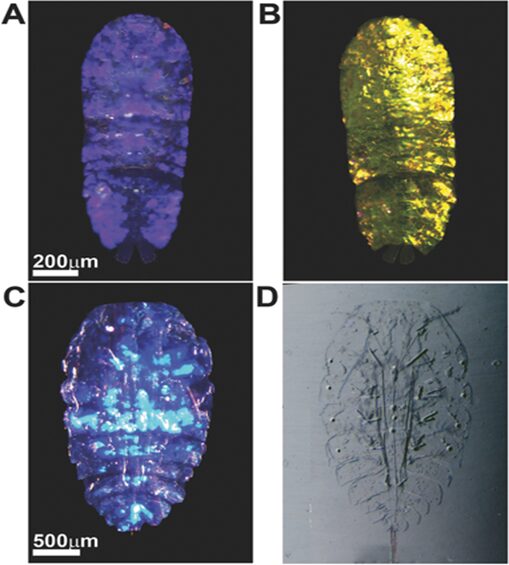
Figure 9: Optical response of sapphirinid males to either dark or light conditions. A) Dark-adapted S. metallina, B) light-adapted S. metallina, C) dark-adapted C. mirabilis, and D) light-adapted C. mirabilis. (Gur et al., 2016).

Another important observation they made is that the incident light intensity was proportional to the rate of the color change. If there was a high intensity, the color change would be as little as 3 minutes and if there was a low intensity, the duration is long and can take up to 9 hours.

Sapphrinid copepods control the reflectance of their guanine plates depending on the incident wavelength. The reflectance represents the percentage of light reflected compared to the incident light. In their research paper, Gur et al studied the changes in the reflectance of Sapphrinid copepods by comparing measured data and Monte Carlo transfer matrix simulations (Gur et al., 2016).

First, the reflectance of the copepod is measured using a custom-built microscope and specialized cameras to capture the image. The objective of the microscope illuminates the slide and captures the reflected light. The collected light is then directed to a CCD camera which produces the image. Based on this image, the reflectance is measured.

As mentioned previously, the copepods control the structural coloration by modifying their cytoplasm spacing. Therefore, the researchers developed a mathematical model to calculate and predict the reflectance based on the wavelength of incident light (Gur et al., 2016). The reflectance is determined by the refractive index and the cytoplasm and crystal thicknesses, so these are taken as parameters. The thickness of a layer is found using Cryo-scanning electron microscopy (Cryo-SEM). The Monte Carlo method involves random repeated sampling; in this case the layer thickness is randomly picked from the Cryo-SEM experimental data for 500 runs. The percentage reflectivity, from which the reflectance is calculated, is found by taking the average of the 500 runs (Gur et al., 2016).

Assumptions taken for the simulation:

The weak dependence of refractive index on wavelength is neglected.
The interfaces of the crystals were parallel.
Normal incident light.

The Monte Carlo Transfer Matrix method involves simulating the reflection of light from the system of guanine plates by considering the randomness in layer thickness. This was accomplished using the formulas (9), (10), and (11) determined by the researchers for the simulation (Gur a al., 2016).

$m_j = \begin{pmatrix}\cos \beta_j & -\frac{i}{n_j} \sin \beta_j \\-i n_j \sin \beta_j & \cos \beta_j\end{pmatrix}\quad \text{where} \quad\beta_j = \frac{2\pi}{\lambda} n_j d_j \quad (9)$

$M_j = \prod_{j=1}^{2k} m_j \quad (10)$

$R = \left| \frac{(m_{11} + m_{12}) - (m_{21} + m_{22})}{(m_{11} + m_{12}) + (m_{21} + m_{22})} \right|^2 \quad (11)$

$n_j = \text{refractive index}, \quadd_j = \text{layer thickness (nm)}, \quadR = \text{reflectivity}$

After completing the simulation and measuring the reflectance experimentally, Gur et al compared the results. As can be seen in Figure 10, by comparing the graphs in Column II and Column III, the simulations and measured results were very similar. This proves that it is a useful and efficient mathematical model. Furthermore, it shows that copepods adapt to their environment by modifying their structural coloration.

Figure 10: The reflectance of sapphirinid copepods. Column 1: Light microscope images of the copepods, Column 2: Measured reflectance, Column 3: The simulated reflectance, Column 4: Cryo-SEM images from which the thicknesses were taken. (Gur et al., 2016)

Conclusion

In conclusion, the remarkable adaptability of copepods reveals itself once again through their adept utilization of mathematical design solutions to optimize their survival behaviors and mechanisms. In response to hydrodynamic disturbances, copepods employ a collective strategy, clustering together which mitigates the impact of disruptive forces. This cooperative clustering is an effective design solution which reduces drag while simultaneously increasing communication and survival. Moreover, copepods center their growth and development around food intake ensuring efficient energy usage. Copepods only begin the molting process once they have accumulated the necessary resources to not waste energy on unsuccessful molting. Furthermore, the modification of cytoplasm spacing between guanine crystals is an innovative mathematical solution finely tuned for adaptive structural coloration. The precision with which copepods adjust in response to light serves both defensive and communicative functions. Vertical migration, an important behavior of copepods, further highlights the role of math in their design solutions. By navigating the waters in pursuit of sustenance and refuge, copepods exhibit a dynamic response to their surroundings. Finally, in low Reynolds number environments, copepods navigate their aquatic habitats with a precision that reflects the optimization of their predator escape tactics.

As we begin to understand the mathematics of copepod behavior and physiology, we gain not only a deeper appreciation for these fascinating organisms but also insights into the interesting, possibly surprising, role of intricate mathematics in the evolutionary optimization of natural design solutions. Through these ingenious solutions, they ensure not only their own survival but their collective one as well. Teamwork makes the dream work. There is no “I” in copepod!

References

Meester, L. (2010). Diel vertical migration. Plankton of inland waters, 651-658.

Peterson, W. (1998). Life cycle strategies of copepods in coastal upwelling zones. Journal of Marine Systems, 15(1-4), 313-326.

Purcell, E. M. (1977). Life at low Reynolds number. American journal of physics, 45(1), 3-11.

Shanbrom, C., Balisacan, J., Wilkens, G., & Chyba, M. (2021). Geometric Methods for Efficient Planar Swimming of Copepod Nauplii. Micromachines, 12(6), 706.

Wroblewski, J. (1982). Interaction of currents and vertical migration in maintaining Calanus marshallae in the Oregon upwelling zone—a simulation. Deep Sea Research Part A. Oceanographic Research Papers, 29(6), 665-686.

Ardeshiri, H., Benkeddad, I., Schmitt, F. G., Souissi, S., Toschi, F., & Calzavarini, E. (2016). Lagrangian model of copepod dynamics: Clustering by escape jumps in turbulence. Physical Review E, 93(4), 043117. https://doi.org/10.1103/PhysRevE.93.043117

Ardeshiri, H., Schmitt, F. G., Souissi, S., Toschi, F., & Calzavarini, E. (2017). Copepods encounter rates from a model of escape jump behaviour in turbulence. Journal of Plankton Research, 39(6), 878–890. https://doi.org/10.1093/plankt/fbx051

Light‐Induced Color Change in the Sapphirinid Copepods: Tunable Photonic Crystals—Gur—2016—Advanced Functional Materials—Wiley Online Library. (n.d.). Retrieved November 27, 2023, from https://onlinelibrary.wiley.com/doi/10.1002/adfm.201504339

Wightman, R. (2022). An Overview of Cryo-Scanning Electron Microscopy Techniques for Plant Imaging. Plants, 11(9), 1113. https://doi.org/10.3390/plants11091113

BERGGREEN, U., B. HANSEN, AND T. KIQRBOE. (1988) Food size spectra, ingestion and growth of the copepod Acartia tonsa during development: Implications for determination of copepod production. Mar. Biol. 99: 341-352.

AMBLER, J. W. (1986) Formulation of an ingestion func- tion for a population of Paracalanus feeding on mixtures of phytoplankton. J. Plankton Res. 8: 957- 972.

Eichner, C., Hamre, L. A., & Nilsen, F. (2015). Instar growth and molt increments in Lepeophtheirus Salmonis (Copepoda: Caligidae) chalimus larvae. Parasitology International, 64(1), 86–96. https://doi.org/10.1016/j.parint.2014.10.006

HAMBURGER, K., AND F. BOETIUS. (1987) Ontogeny of growth, respiration and feeding rate of the freshwater Calanoid copepod Eudiaptomus graciloides. J. Plank- ton Res. 9: 589-606.

HARRIS, R. P., & PAFFENHOFER (1976) Feeding, growth and reproduction of the marine planktonic copepod Temora ZongicornisMiiller. J. Mar. Biol. As- sot. U.K. 56: 675-690.

PAFFENHER, G. A. 1971. Grazing and ingestion rates of nauplii and adults of the marine planktonic co- pepod Calanus helgolandicus. Mar. Biol. 11: 286-298.

Santer, B., & Van den Bosch (1994) Herbivorous nutrition of CycZopsvicinus: The effect of pure algal diet on feeding, development and reproduction and life cycle. J. Plankton Res. 16: 171-195.

van den Bosch, F., & Gabriel, W. (1994). A model of growth and development in Copepods. Limnology and Oceanography, 39(7), 1528–1542. https://doi.org/10.4319/lo.1994.39.7.1528