The Mathematics of Tardigrade Behavior and Development
Luccia Jabbour, Eden Karp-Foster, Jeremy Lachance, Wadi Zahka
Abstract
Tardigrades are equipped with a plethora of features that, most notably, allow them to cope with very harsh conditions that very few organisms are known to be able to withstand. In addition to these tools themselves that they possess, tardigrades' peculiarity can also be assessed by models that successfully represent their morphological special characteristics and predict quite accurately their interspecific behavior, that is the decisions that they make while foraging. For one, tardigrades exhibit allometric traits, meaning that the relative sizes of their body parts cannot be linearly correlated with each other and that the volumes of their internal organs are unusual, thus permitting their contraction when entering the tun state. Tardigrades, moreover, follow an apparent algorithmic approach when it comes to prey, depending on many factors such as prey density or their buccal morphology. Although these latter models may seem to be more related to the pure science of biology rather than to engineering, they are still arguably relevant for the field of bioengineering since they could be useful in the context of biomimicry, notably, knowing that they depict optimums reached to after millions of years of evolution that could be relevant for implementing into microrobots behaving similarly to living organisms in terms of energy uptake or subsistence in various microenvironments, if ever that comes to exist, as optimal algorithms.
Introduction
Tardigrades, also known as “water bears” or “moss piglets”, are very small invertebrates and close relatives to arthropods that belong to the phylum Tardigrada. They were first discovered in 1773 by Johann August Ephraim Goeze, who named them “water bears” due to their bear-resembling movements. Three years later, Lazaro Spallanzani modified their name to “Tardigrada”, meaning “slow stepper” (Macdonald, 2004).
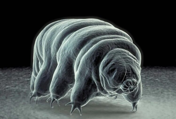
Figure 1: Scanning electron micrograph of a tardigrade (Britannica, 2023).
Tardigrades are characterized by their short and plump barrel-shaped bodies with lengths spanning from 0.05 mm to 1.2 mm (Weronika, 2017). They possess four pairs of limbs, each ending in four to eight claws or suction disks. Similarly to the exoskeleton of insects and arthropods, tardigrades have a tough cuticle that covers their body. Moreover, tardigrades undergo molting to shed their cuticle during growth, which is akin to the behavior of some arthropods. Their body is also divided into two parts: a head region and a body. The head is composed of a tubular mouth encircled by stylets used for piercing plant cells, algae, and other organisms for sustenance. From the mouth extends the buccal tube, a rigid sclerified structure of the tardigrade feeding apparatus. The feeding apparatus consists of a buccal ring connected to a straight buccal tube, a buccal crown, longitudinal thickenings within the pharynx, and a stylet system composed of piercing stylets within stylet coats, and stylet supports (Surette F, 2023). The buccal-pharyngeal apparatus has smaller parts that contribute in such a way that the movement of the apparatus is entirely supported. Furthermore, the buccal tube serves as a conduit for ingesting food while the pharyngeal bulb, located at the base of the buccal tube, is responsible for grinding the food (Guidetti, R et al., 2013). The body cavity of the tardigrade is a hemocoel filled with fluid, serving as a medium for oxygen and water transport as tardigrades lack specialized organs for respiration or circulation.
Their brains are bilaterally symmetrical, paired with neuron clusters, and are connected to a large ganglion below the esophagus, giving rise to a double ventral cord that extends throughout the body. The ventral cord contains ganglions on each segment of the body whereas lateral nerves extend towards the limbs. Many tardigrades exhibit a pair of compound cup-shaped eyes and sensory bristles distributed across their head and their body. Reproductively, tardigrades demonstrate diverse strategies. Typically oviparous, these microorganisms mostly engage in external fertilization, where the female molts to lay eggs fertilized externally by the male. Some species, however, opt for internal fertilization, with the male depositing sperm inside the female's cuticle, thus showcasing variation in their reproductive methods.
Tardigrades, known for their polyextremophilic nature, exhibit incredible resilience in diverse ecosystems that range from mountain peaks, deep seas, and volcanic regions to intertidal zones, deserts, urban landscapes, and even ice niches in the Arctic (Reyes et al., 2023). While they thrive in various environments, freshwater mosses and lichens remain their preferred habitats. What makes the tardigrades ripe for research is, notably, their ability to withstand very harsh and extreme environments, such as challenging terrains with regard to their microscopic size, highly fluctuating conditions, rapidly changing humidity, and extreme temperatures. As it will be conveyed nevertheless herein, tardigrades turn out to be very interesting as well in some of the models that characterize them.
Their remarkable endurance in hostile environments essentially stems from their capacity for cryptobiosis, a state of reduced metabolic activity and desiccation (Macdonald, 2004). The adaptability of tardigrades has intrigued researchers, leading to experiments like those conducted by the European Space Agency, where two tardigrade species, Richtersius coronifer, and Milnesium tardigradum, were sent into low Earth orbit during the FOTONM3 mission, enduring exposure to space vacuum and UV radiation and remarkably surviving (Jönsson, 2008).
In this paper, we tackle different aspects of tardigrades drawn through a mathematical perspective, that is the study of some foraging models characterizing their predation approach along with the study of their allometric traits and their geographical distribution.
The interspecific interactions of tardigrades described as a mathematical model
Tardigrades are, from an objective point of view, among the simplest multicellular organisms. They are microscopic, or at least very small, animals that possess a relatively rudimentary nervous system. In fact, their brains are expected to contain fewer than 200 neurons (Mayer et al., 2013). Thus, tardigrade behavior is also not expected to be governed by complex or even conscious and thoughtful reasoning, but rather by simple principles that could be modeled as algorithms. More strikingly, tardigrades' nervous system comprises a prominent ring nerve surrounding the buccal tube (Fig. 2 and 3) that is highly linked to the brain besides innervating both the peribuccal lamellae, near the mouth opening, and the stylet apparatus. The stylet apparatus is a system composed of muscular fibers and CaCO3, which allows tardigrades to pierce the body walls of prey items and to suck their content for feeding (Guidetti et al., 2013). An important innervation in both of these structures is essential for tardigrades, as they detect the presence of prey, which they can assumably hardly see, by labial contact (Hohberg & Traunspurger, 2009).

Figure 2: The Nervous System of Macrobiotus harmsworthi. A: Ventral view, showing four ganglions ga, a dorsally situated brain, linked by pair somata free connectives (red, labelled with antibodies specific to α-tubulin) and composed of neurons (nuclei in green). B: Lateral view. C: Anterior end in ventral view. D: Anterior end in dorsal view. The asterisks and arrows point towards the aforementioned ring structure. Legend: br = brain, cn = connectives, ga1-ga4 = trunk ganglia (1-4), il = inner brain lobe, le1-le4 = walking legs (1-4), np = central brain neuropil, oc = outer connective, ol = outer brain lobe, ml = median brain lobe, so = neuronal somata. Scale bars: 25 μm (A), and 10 μm (B-D). (Mayer et al., 2013).
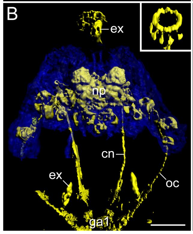
Figure 3: Detailed View of Macrobiotus harmsworthi's brain structures. In blue: autofluorescent brain contours. In yellow: immunolabelling of connective structures. A ring structure near the buccal apparatus can easily be observed and is brought out in the schematic. Legend: as = anterolateral sensory fields, bd = neurite bundles innervating the stylet musculature, cn = connective, co = commissure of the stomodeal complex, ga1 = first trunk ganglion, ln = leg nerves, mp = macroplacoids, ne = neurites supplying the peribuccal/mouth lamellae, np = central brain neuropil, oc = outer connective, pn = peripheral nerve, ps = posterolateral sensory fields, un = unpaired posterior nerve/neurite. Scale bars: 20 μm (A-D). (Mayer et al., 2013).
In some way, however, despite tardigrades' brains' simplicity, invertebrates' and vertebrates' nervous systems are known to function analogously to each other when it comes to finding and applying cost-benefit solutions, which are what is at stake when tardigrades are exposed to food sources in their environment. Indeed, it is well underlined that the “appetitive state [in both vertebrates and soft-bodied invertebrates] determines action responses from a repertory of possibles and transmits the decision to a premotor system that frames the selected action in motor arousal and appropriate postural and locomotion commands” (Gribkova, 2023). Tardigrades have been demonstrated to obey, through that process, certain definite mathematical laws in the context of foraging (Hohberg & Traunspurger, 2009; Jeschke & Hohberg, 2008), which, as it will be explained further on, are optima (in the sense that they contribute to maximizing biomass gain with respect to many different factors) and constitute therefore important design solutions for coping with highly fluctuating food availability that come along with highly fluctuating environments. Indeed, being faithful to such algorithmic laws developed throughout evolution is essential for tardigrades, as most of their prey are not distributed evenly across a certain environment, with a variation of food quantities by a factor of 200 within a few cubic millimeters of soil (Hohberg & Traunspurger, 2009).
Tardigrades' predictable selection of prey items
Tardigrades can be exposed to many different kinds of prey in their environments, such as plant cells, algae, bacteria, protozoa, small invertebrates like nematodes and rotifers, and even other tardigrades of distant phylogenetic genera (Roszkowska et al., 2016), all of which can be of different sizes. With regards to such a high diversity of food sources, tardigrades should, according to the foraging theory (Stephens & Krebs, 1986), strive to maximize energy uptake per time while considering both benefits and costs, which depend on the prey itself, that is on their size, on their energy value, on their response to being preyed on or their handling time, for instance, as well as on the environmental constraints, that is prey densities, most notably (Hohberg & Traunspurger, 2009).
In one study, Macrobiotus richtersi's prey exploitation and prey selectivity with respect to prey size and density, where the prey is the bacterivorous nematode Acrobeloides nanus, is investigated (Hohberg & Traunspurger, 2009). Two sizes of prey are herein distinguished, that is type A1 and type A2, whose mean wet mass and mean body length are respectively mA1 = 28 ng, LA1 = 220 µm, mA2 = 20 ng and LA2 = 300 µm, and which also differ in required handling time. Also, tardigrades' biomass gain depends on the size of a prey item they feed on and the degree at which it is consumed.
The first relevant observation noted was that when A2 prey type's abundance was above a certain threshold, tardigrades systematically preferred this type over the other. The prey's degree of consumption has been shown to be correlated with the availability of food as well as with the ratio of biomass extraction to the time invested in searching and handling. For assessing this relationship, two four-hour experiments (A and B), both involving one three-days starved tardigrade, have been performed; the first one (A) solely with A2 nematodes at eleven different densities (10, 25, 50, 75, 100, 150, 200, 250, 300, 350, and 400), and the second one (B) with various ratios r of A1 and A2 prey types (1:9, 3:7, 5:5, 7:3, and 9:1).
Some parameters have been defined, with i standing for type A1/A2, which are the prey density Ni, the prey encounter rate βi (number of encounters for the predator, that is ten, divided by the prey density and the time taken), the predator encounter rate αi, the mean time in seconds for search for a prey item TSi, the number of attacks recorded di, and the preference for a certain type of prey, which will here be denoted as preference, simply. No matter the prey density, βA1 = 0.64/hr and βA2 = 1.90/hr have been observed. Also
α_i=β_i×N_i
T_{Si}=3600/(β_i×N_i )=3600/α_i Preference=ln[(N_{A2}-d_{A2})/N_{A2} ]/ln[(N_{A1}-d_{A1})/N_{A1} ] +ln[(N_{A2}-d_{A2})/N_{A2} ].The latter equation corresponds to Manly's formula (Manly, Miller, & Cook, 1972), which is adequate as it takes prey depletion into account.
A pre-experimental hypothetic model
While A1 prey was always swallowed by Macrobiotus richtersi in a linear manner, A2 prey was either left at some time point P, as pictured in Fig. 4, or swallowed after sufficient piercing and sucking and thus consequent reduction of their body size. This point P represents a predicted optimum with respect to 1) the biomass gain and 2) the time invested in searching for and feeding on a prey item. It is also predicted that, in the context of experiment A, it would depend on TS-A2 and that in the context of experiment B, it would also depend on the latter ratios r.
Continuing with the predictions made, point P would, in context A, relate to the following equation, where t is the same independent variable as in Fig. 4 displaying y(t):
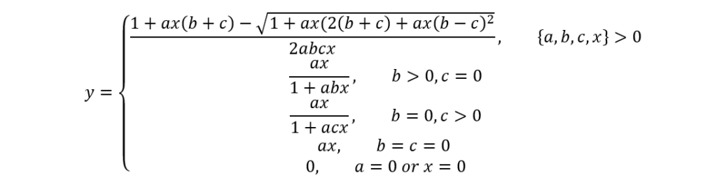
P=y(t)/(t+T_{Si} )=6.9349t/((1+0.0754t)(t+T_{Si}))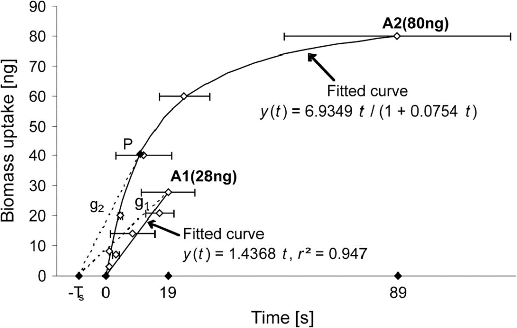
Figure 4: Feeding rate of Macrobiotus richtersi preying on Acrobeloides nanus, as its biomass uptake y with respect to the time spent consuming the nematodes A2 and A1 (we will refer to the function as being y(t)). As it can be observed, the point P constitutes a predicted optimum and the curve corresponding to A2 satisfies the equation y(t) = 6.9349t/(1+0.0754t) (Hohberg & Traunspurger, 2009).
As for in context B, the following more complex equation introduces the parameter r (same as mentioned)[1] as well as some other better estimates the point P:
P=(r_{A2} y_Q+(1-r_{A2} ) m_{A1})/(r_{A2} t_Q+(1-r_{A2} ) T_{FA1}+T_S )mA2 here stands for the mass of the smallest prey (in this case 28 ng), yQ and tQ together relate to “when to leave a prey item A2 under the optimal policy” (Hohberg & Traunspurger, 2009), which is essentially the maximum value of the simple derivative y'(t) = dy/dt of the function y(t) given above, and finally TFA1 stands for the mean time required for consuming a prey item A1.
Verification of the latter pre-experimental hypothetic models
After experimentation A, it was revealed, consistently with the latter predicted model, that prey items were consumed more with increasing search times; indeed, tardigrades devote more time for a single prey item at large TSi, perhaps as it is uncertain for them whether they will easily encounter a satisfactory quantity of prey items afterward. On the other hand, they spend less time on each one of them with lower TSi, this time perhaps, as we hypothesize again, in order to accumulate food reserves in case this profitable abundance of food is merely temporary. The observations made in experiment A are compiled and displayed in Fig. 5.
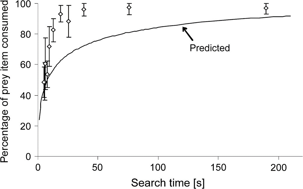
Figure 5: Percentage of prey items consumed with respect to search time TSi. White points correspond to empirical data whereas the traced curve corresponds to the predicted model as given in Fig. 4 (Hohberg & Traunspurger, 2009).
In fact, it was concluded that these empirical data are closely related to the predicted model for a narrow window of low TSi (from about 5-9 s). However, for longer, and most search times in general, biomass exploitation was even more important than predicted, though, the tendency predicted was roughly accurate along with the empirical curve. This first function as traced in Fig. 5 constitutes the first optimum that has been observed in tardigrades when only the variable of search time was present. Nonetheless, more observations made allow for the statement of a broader and more overall design solution that encompasses other variables as well, as this will be developed further on.
As for experiment B, no preference whatsoever for the A2 type was recorded, contrarily to the predictions that were reasonably made; in fact, the main preference value Preference = 0.462 ± 0.046, which is nearly null, is displayed by the almost linear relationship represented in Fig. 6. However, the larger A2-type prey there is, the lesser percentage of a prey item is consumed, which is comprehensible and consistent with experiment A, in which tardigrades seem to take advantage of the profitable situation of abundance by killing as much prey as possible to apparently make food reserves.
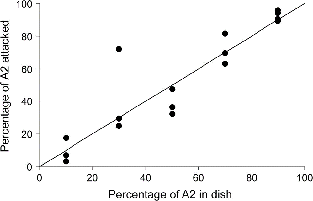
Figure 6: Nearly linear function with the percentage of A2-type prey items present as the independent variable and the percentage of A2-type prey items attacked as the dependent one, which describes a nearly null preference for the A2-type prey over the A1-type one (Hohberg & Traunspurger, 2009).
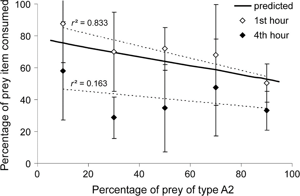
Figure 7: Percentage of one prey item consumed with respect to the percentage of prey of type A2 present. Points represent empirical data whereas the curve is a prediction of the latter function and represents the percentage of prey biomass gained plotted against the percentage of prey of type A2 present. (Hohberg & Traunspurger, 2009).
It is noteworthy that, as tardigrades detect prey items by tactile contact with their circumoral field surrounding their buccal apparatus and not by sight, it might indeed not be possible for them to express any preference regarding types of prey. What is surprising and poorly understood concerning tardigrades in particular and compared to other organisms, though, and which is also one main topic of Hohberg's study, is how they access information regarding prey density. In their case, it is yet essential that they be able to do so, as akin to most other environmental conditions that they face (e.g., temperature, UV exposure, moisture, etc.), prey density significantly varies within their natural habitats. In fact, nematodes, just for instance, aggregate in nutrient-rich hot spots in soils, such as in the rhizosphere, and are less concentrated in other places. Thus, food quantities available for tardigrades may differ, as mentioned, by a huge factor of 200 within only a few cubic millimeters of soil. Hohberg was unable to adjudicate on tardigrades' ability to detect chemical cues in their environments, so it appears that tardigrades rely on their experience and respond in algorithmic ways by adopting the behaviors observed in the experiment, depending on the information they get from how frequently they encounter prey items. Returning to tardigrades' nervous system, this possible decision-making capability is quite startling considering the relative elementarity of tardigrades' brains compared to more advanced vertebrate predators' nervous systems, notably.
Three complementary models for describing tardigrades' foraging behaviors
Three other models have been tested for assessing tardigrades' foraging behaviors (Jeschke & Hohberg, 2008) and will hereafter be briefly described. The first one is the Holling's equation, which corresponds to the following:
y=(βγδε×x)/(1+βγδε×x×(t_{att}/ε+t_{eat} ) )=ax/(1+abx)y is the number of prey items consumed, x the food abundance (per area or volume), a the consumer success rate, and b the consumer handling time per prey item. a and b are further developed in other parameters which are β, the same encounter rate as in Hohberg's experiment, γ, the probability that the consumer attacks do detect prey δ, ε, the attack efficiency (or frequency of successful predation events), tatt the attacking time, and teat the consuming time.
Although Holling's equation integrates many pertinent parameters, it does not consider tardigrades' satiation state, which the second model (named SSS by Jeschke & Hohbergh), including the same parameters with, in addition, c, does:
c=st_g
The c parameter here accounts for the digestion time, and s and tg respectively stand for the “reciprocal capacity of the hunger-determining part of the gut”[2] (Jeschke & Hohberg, 2008) and for the gut retention time. Again, the SSS model is convenient and elaborate; however, it assumes that tardigrades' hunger level remains constant, which is a significantly simplified abstraction, knowing that it is actually very changing due to the highly variable nematode densities in tardigrades' environments, hence the application of the proposed so-called satiation model comprising three essential equations and which considers the depletion of prey items with time as well as a non-constant hunger level (at the expense of an even greater complexity):
(dy(t))/dt=(h(t)ax(t))/(1+h(t)abx(t))
x(t)=x(0)-y(t)

The satiation model essentially states that the rate at which the number of prey items is consumed is moreover proportional to the predator's hunger level h3, that the food abundance x decreases proportionally to the number of prey items eaten, and that the hunger level variation is increased by digestion (sub-equations 1 and 2) and is decreased by ingestion (sub-equation 3). It has been demonstrated that this third model best characterizes tardigrades' foraging behaviors after carrying out a similar experience to Hohberg's in principle. The curves corresponding to the three previous models are compared in Fig. 8, where the satiation model's better accuracy is easily assessable.
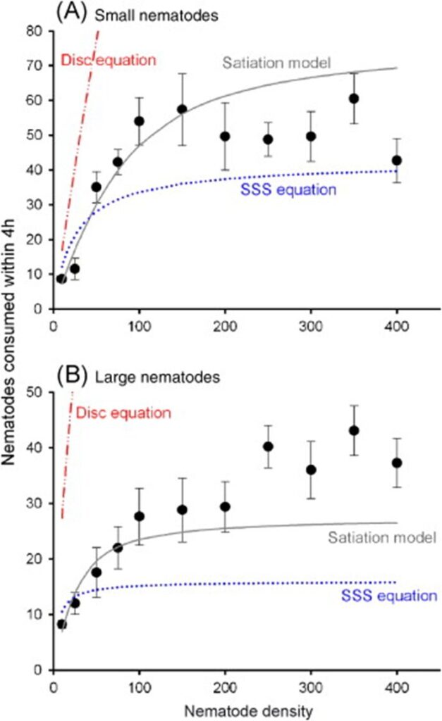
Figure 8: Comparison of the curves corresponding to the three models described with actual empirical data, for both small and large nematodes, presumably respectively similar to A1 and A2-type nematodes (Jeschke & Hohberg, 2008).
Overall, tardigrades' foraging behaviors are quite predictable and appear, as mentioned, to follow an algorithmic decision-making process requiring very minimal intelligence according to the limitations of their rudimentary nervous system. In that first sense, the algorithms that tardigrades are faithful to are optima with respect to their limited brain capacities and are thus design solutions. After experimental investigation, it has been demonstrated that the “satiation model” proposed by Jeschke & Hohberg, which encompasses several environmental and organismal variables such as, only to name a few, the hunger level, the food abundance, and the consumer handling time per prey item, seems to be the closest to empirical observations. Other characteristic curves have been described when observing tardigrades preying on nematodes with respect to different percentages of larger ones over smaller ones (A2-type vs. A1-type) and with respect to different searching times correlating with prey densities. Such predictable behavior from tardigrades is likely to be a design solution in the context of the emphasized high variability and uncertainty of prey densities in their natural ecosystems and in the sense that it strives to grant them optimal net gains in all circumstances.
Buccal morphology of tardigrades as a function of optimization
Microfauna (organisms like tardigrades, rotifers, nematodes, etc.) is extremely important. These organisms inhabit diverse environments like soil, water systems, and cryptogams (plants like mosses, algae, and lichens). Microfauna plays an essential role in the intricate micro food web, acting as mediators in nutrient cycling between bacteria, fungi, microorganisms, and plants (Nelson, 2002).
These microorganisms affect the rate of nutrient cycling in various ways. Microbivorous microfauna directly impact bacterial, archaeal, and fungal communities by consuming them, thereby releasing nutrients. On the other hand, carnivorous and omnivorous microfauna participate in nutrient cycling by preying on other members of the microfaunal community. Tardigrades are especially important, especially those in limnoterrestrial habitats (soil and moss cushions), which play roles as both prey and predators in these ecosystems. The regulatory function of tardigrades is influenced by various factors, including their abundance, environmental conditions, density of prey, and feeding preferences, which are not thoroughly understood (Hohberg, 2005). Understanding the feeding preferences of organisms is often determined by their morphological traits or the anatomy of their feeding structures. In the case of tardigrades, their classification into different feeding groups (herbi-, omni-, and carnivores) is based on and related to the structure of their buccopharyngeal apparatus, specifically the buccal tube (Roszkowska et al., 2016).
Conditions of the study
In order to understand the behavior of the tardigrades in relation to their food preferences, the feeding preferences of nine predatory tardigrade species concerning three types of microfaunal prey: nematodes, rotifers, and small herbivorous tardigrades were studied. These nine tardigrades had different tube dimensions for their feeding preferences on three types of microfaunal prey. The size of the buccal tube is represented in Fig. 9 (Tůmová, 2021)
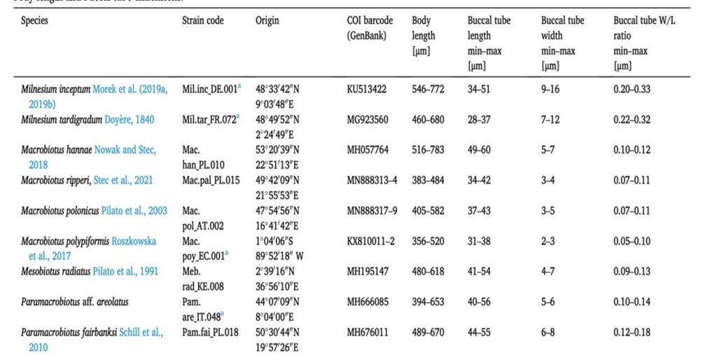
Figure 9: Tardigrade species used in the study and the ranges of body length and buccal tube dimensions (Tůmová, 2021).
Methodology used in analyzing the data related to the feeding preferences and consumption behaviors of predatory tardigrades
Constrained Redundancy Analysis (RDA) is a statistical technique used to explore relationships between response variables (in this case, the feeding preferences and consumption rates of predatory tardigrades) and explanatory variables (such as the characteristics of the tardigrades: body length, buccal tube length, width, buccal tube width/length ratio, etc.).
Since both the response variables and explanatory variables were multivariate (consisting of multiple variables or traits), constrained RDA was employed. This analysis allows researchers to assess the differences in the data while considering multiple variables simultaneously. Multiple RDA analyses were performed successively to answer different research questions. The first analysis aimed to assess whether the differences in the consumption rate (total number of consumed items of each prey type) could be better predicted by buccal tube dimensions or by the identity of the predator species. The second analysis sought to determine whether the relative preferences of the tardigrades for different types of prey could be better predicted by buccal tube dimensions or by predator species identity. The third analysis aimed to investigate if buccal tube dimensions could explain variations in preferences within species (intraspecific variability) and whether these traits could predict the overall prey preferences of the species (ter Braak & Smilauer, 2012).
Behavior of predatory tardigrades in relation to their food preferences and consumption rates
The preference for predatory tardigrades depended more on their functional traits. When evaluating the proportional differences between the three types of prey among the total number of consumed prey (relative preferences), morphometric traits of the tardigrades were more useful for understanding the food preferences. In fact, both morphometric traits combined with species identity explained 18% of the variation of the relative preferences, with 1% on the consumption rate and 17% on the morphometric traits (tubal length accounted for 11% of the variation, buccal tube ratio and width explained 4% and 2% respectively) (Tůmová, 2021).
Moreover, the ordination diagram (Fig. 10) shows that the buccal tube length corresponds with the first ordination axis (x-axis), whereas buccal tube width and buccal tube width/length ratio are represented by the second ordination axis (y-axis). Upon examining the diagram, it is evident that among predatory tardigrades, tardigrade prey was generally the least favored choice. However, those tardigrade predators possessing longer buccal tubes demonstrated a higher frequency of consuming tardigrade prey compared to tardigrade predators with shorter buccal tubes. Simultaneously, all tardigrade predators showed a preference for nematode prey. Nonetheless, tardigrades with shorter buccal tubes had a diet consisting of a larger proportion of nematodes compared to tardigrade predators with longer buccal tubes, as depicted in Fig. 11 and 12 (Tůmová, 2021).
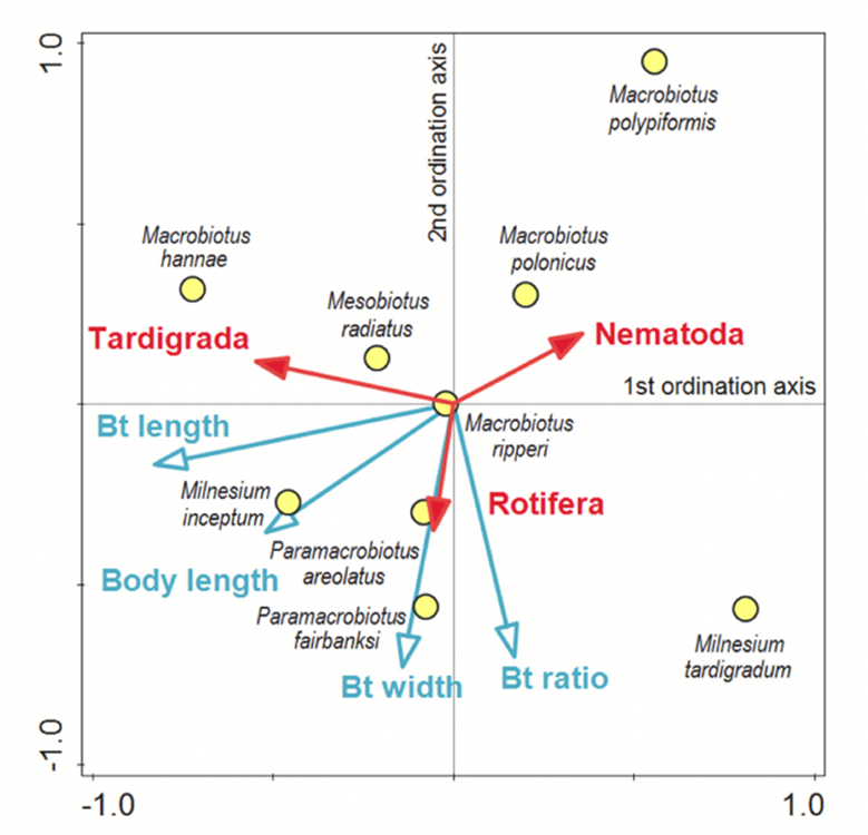
Figure 10: Ordination diagram of Constrained RDA (the blue arrows represent the direction of increasing value of measured traits, whereas the red arrows represent the direction of an increasing percentage of the three types of consumed prey. Finally, the yellow points represent the position of species that agree the best with their feeding preferences (Tůmová, 2021).
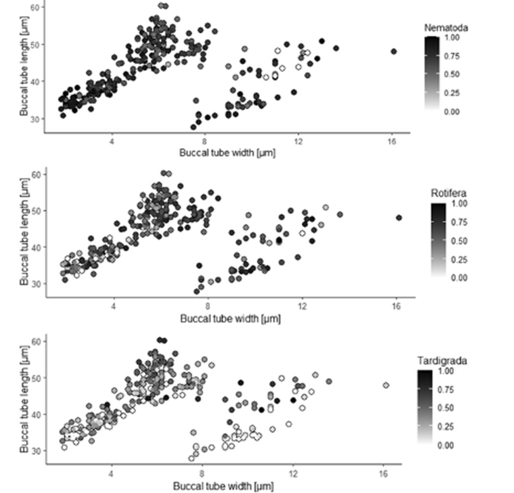
Figure 11: Percentage of consumed nematodes, rotifers, and tardigrades respectively, and the relationship with buccal tube dimensions (Tůmová, 2021).
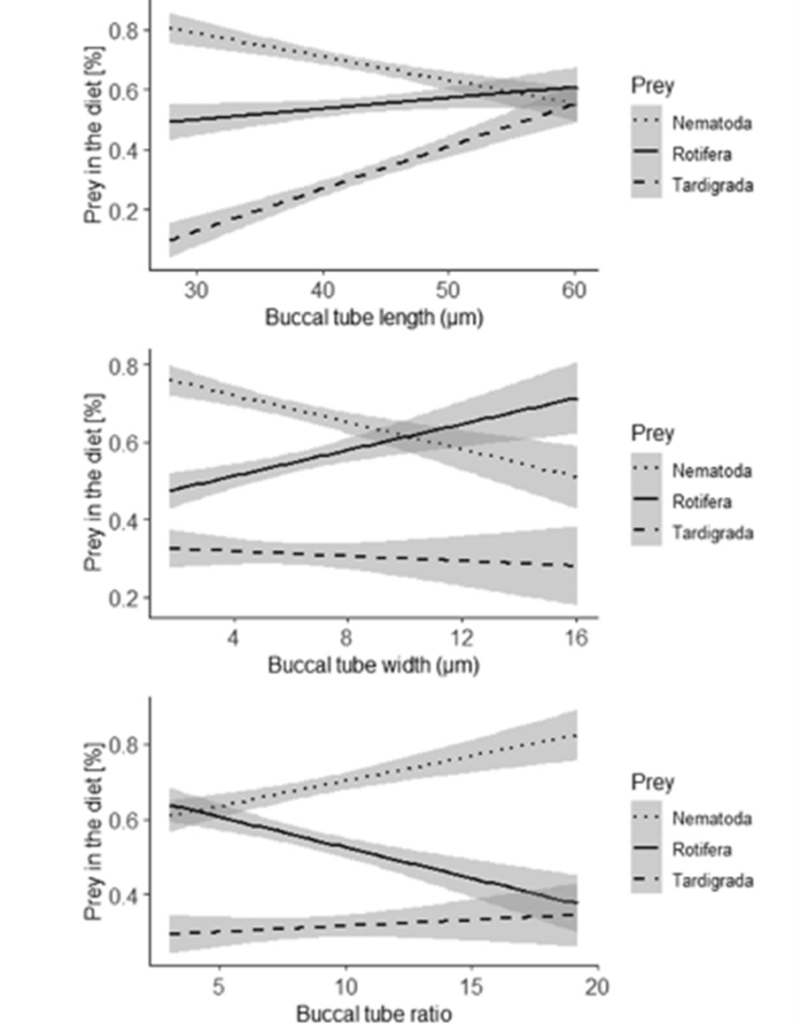
Figure 12: Relationships of dimensions of the buccal tube length, buccal tube width, and buccal tube ratio (in micrometers) to the proportions of the three types of prey in the diet of predatory tardigrades with 95% confidence intervals for the regression lines represented by the grey band around the linear representations (Tůmová, 2021).
In conclusion, buccal tube dimensions can indicate the preferences of predatory tardigrades. However, for a more comprehensive understanding of predatory tardigrade preferences, several additional factors warrant consideration. It is important to expand the testing parameters to achieve a more thorough understanding, and it is crucial to include tardigrades exhibiting a broader range of body and buccal tube dimensions in preference tests. Moreover, evaluating tardigrade preferences in their natural habitats rather than only in controlled laboratory conditions is necessary. It is also crucial to explore preferences among other groups that serve as potential food sources for tardigrades. However, this can already help shed light on the interactions existing between tardigrades and other microfaunal groups in the micro food web (Tůmová, 2021).
The elimination of body size effects in the study of allometric traits in tardigrades
In the study of quantitative traits in organisms across the animal kingdom, researchers often come across the particular problem of the variability of morphological traits due to bodily size – in addition to a specific external factor that they are trying to study (Lleonart et al., 2000). When attempting to identify and quantify this external factor, it is necessary to remove the effects of body size on the measured values in the sample space. Historically, this has been accomplished via the outright removal of outlying specimens from the sample pool (specimens that are “unusually large” or “unusually small”) (Pilato, 1981; Peluffo et al., 2007). This allows the researchers to compare only specimens of a similar size and disregard body size effects.
However, this is not a viable solution. For one, it is difficult to procure enough specimens of similar size, particularly in species that inhabit inaccessible environments. Additionally, the removal of entire groups of specimens of a size outside a particular range means that unusually large or small specimens are completely eliminated from consideration of quantitative traits. Introducing such selection bias has the potential to drastically affect the results of the study of these traits.
Consequently, new methods of removing the effects of body size must be developed to allow for the comparison of morphological traits across specimens of varying sizes. This is particularly dependent on the type of trait being studied, and how it changes in relation to changes in body size.
Isometric vs allometric traits
The relationship between the size of various traits and body size is generally classified into two categories: isometric and allometric traits, governed either by isometric or allometric growth. In the case of isometric growth, the change in body size is proportional to the change in the trait being studied. As body size increases by 1 unit, the trait changes by k units. In allometric growth, on the other hand, traits do not change proportionally to body size, meaning that as body length increases, the traits do not change at a constant rate (Shingleton, 2010).
In the case of isometric growth, the issue of body size removal can be resolved simply by expressing the trait as a proportion of body size. As a result, the effects of body size on the comparison of different specimens are eliminated because it is not quantitative values that are being considered, but rather the trait as a ratio or percentage of its own body size. For instance, in the comparison of limb lengths of different specimens, it may be found that one specimen's average limb length is 4 µm larger than the other, but both have an average limb length of 80% of their body length.
It is much more difficult to remove body size effects from data collected on allometric traits because their relationship is not governed by a constant. For instance, in eutardigrades, the body size is proportional to the length of the buccal tube, but body length is more variable due to the flexibility of the cuticle and the orientation and coverslip pressure on the specimen” (Bartels et al., 2011).
As a result, more complex normalization techniques must be developed in order to remove body size effects of allometric growth and allow the comparison of quantitative morphological traits independent of body size.
In the study of tardigrade morphology specifically, both pt indices and Thorpe's normalization are regularly employed to remove body size effects, with varying levels of success.
PT indices
Over the past few decades, the use of pt indices to remove body size effects in tardigrades has become relatively standard practice. The pt index is defined as the ratio of a measurable trait to the buccal tube length, as a percentage (Pilato, 1981). It is believed that using the buccal tube length provides more consistent data because the buccal tube is a hardened, or “sclerotized,” structure, meaning it is “less prone to curvature and distortion from preservation and mounting techniques” (Bartels et al., 2011). The morphology of the buccal apparatus is shown in Fig. 13 and 14.
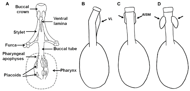
Figure 13: The buccal apparatus in tardigrades, comprising the buccal crown, buccal tube, and buccal-pharyngeal basket. (A) Ventral view (B-D) Lateral view of varying types of bucco-pharyngeal strengthenings; VL: ventral lamina, AISM: apophyses for the insertion of the stylet muscle (Bingemer & Hohberg, 2017).
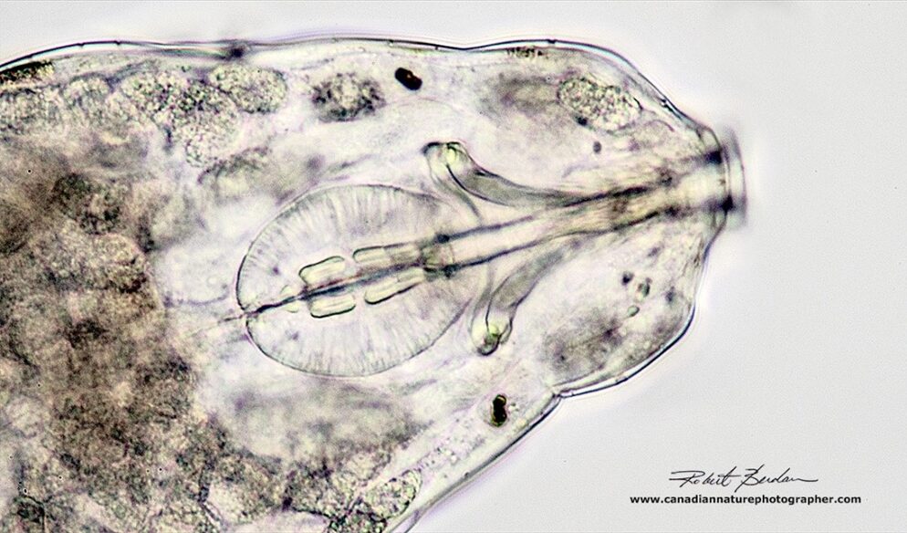
Figure 14: Closeup of tardigrade via bright field microscopy at 400X. Note the buccal-pharyngeal apparatus in the center and the buccal tube on the right (Berdan, 2018).
However, the use of pt indices has clear limitations. Since the index is only a proportionality constant, it is effective for cases of isometry, but it is not very useful for the study of allometric traits because it implies a proportional, linear relationship between the trait and buccal tube length (Bartels et al., 2011). As a result, exponential relationships have been developed to describe allometric cases and allow for normalization.
The allometric model and Thorpe's normalization
A general equation relating two allometrically related magnitudes X and Y in a body is given by:
Y=αX^β
In this equation, α and β are parameters. In particular, α is known as the “coefficient of shape” because its value depends on the shape of the organism's body, while β is the coefficient of dimension, transforming X from the dimension of Y to a new dimension, β (Lleonart et al., 2000). For the elimination of body size effects, Y is set as the body size.
This equation gives rise to several fascinating relationships between body size and traits. When β = 0, the trait is independent of body size. When β=1, the relationship is in fact isometric, not allometric, since X and Y are now related by a proportionality constant α. When β<1, the relationship is negatively allometric (decreasing as body size increases), and when β>1, the relationship is positively allometric (increasing as body size increases). As a result, the equation has a broad number of applications in the study of morphology – not just in cases of allometry.
This relationship can be linearized via a regression of a log-log transformation, which also has the effect of reducing skewness in the normal distribution of the equation (Feng et al., 2014). The new equation is as follows:
log(Y)=log(α)-β[log(X) ]
From this, Thorpe (1975) developed a normalization technique that removes the effects of bodily size from calculations. Note that a and b are used interchangeably with α and β.
Y^*=10^{log[Y_i-b(log(X_i)-log(X_0 ) )] }According to Bartels et al., “Y* is the Thorpe normalized trait, Yi is the individual measurement of the quantitative trait, Xi is the corresponding individual measurement of body size, Xo is mean body size and b is the slope of the regression line for the log–log-transformed data” (2011).
Lleonart et al. (2000) further simplified the equation to the following:
Y^*=Y_i [(X_0 )⁄X_i ]^b
Thorpe observed that the equation has the property of transforming the quantitative trait measurements, Yi , to the values Y* they would assume if each specimen were of mean body size Xo. In fact, “this normalization was shown to be more effective than other statistical techniques that correct for body size” (Reist, 1985).
Thorpe normalization vs PT indices
In 2011, Bartels et al. compared the results of using pt indices and Thorpe normalization on the study of several traits, including internal buccal tube width (BTWI), claw length (CIE), and distance between stylet support points (SSA). These measurements as a function of body length are shown in Fig. 15 below.
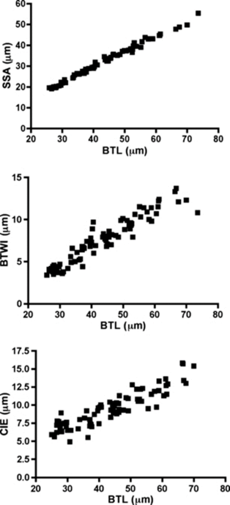
Figure 15: Internal buccal tube width (BTWI), claw length (CIE), and distance between stylet support points (SSA) plotted against buccal tube length (BTL) for Paramacrobiotus tonollii (Bartels et al., 2011).
The researchers then performed a log-log regression on the data to linearize it, as shown in Fig. 16.
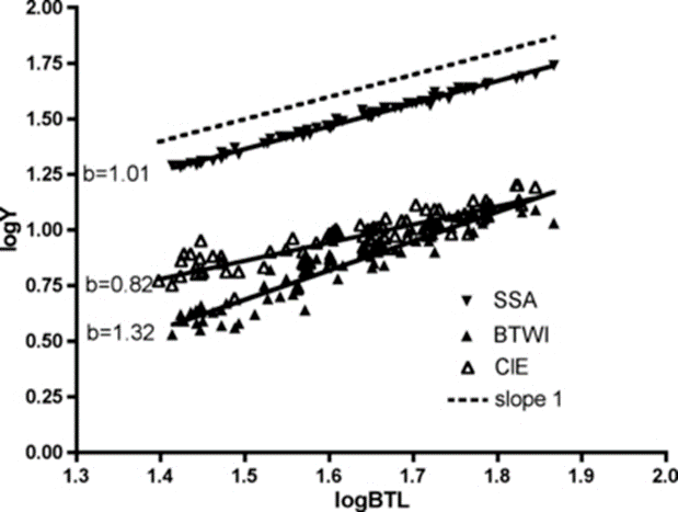
Figure 16: Log-log plot with linear regression of internal buccal tube width (BTWI), claw length (CIE), and distance between stylet support points (SSA) vs buccal tube length (BTL) for Paramacrobiotus tonollii (Bartels et al., 2011).
Finally, the researchers performed both pt indexing (Fig. 17) and Thorpe normalization (Fig. 18) on the log-log regression and compared the results. They deduced that Thorpe normalization was more successful at removing body size effects since it led to lines whose slope was nearer 0 for each trait (i.e. that demonstrated less change as over change in body size). In fact, for the Thorpe normalization, it was found using a p-test of significance that “none of these slopes [were] significantly different from a slope of 0 (F < 0.316, p > 0.57).” Meanwhile, for pt indices, “the slopes were significantly different from 0 (F > 285.3, p < 0.0001)” for all traits” (Bartels et al., 2011).
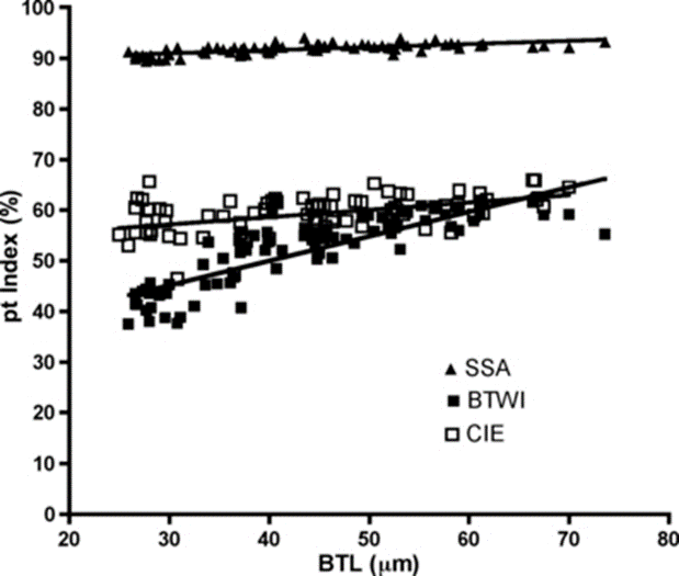
Figure 17: pt index of internal buccal tube width (BTWI), claw length (CIE), and distance between stylet support points (SSA) vs buccal tube length (BTL) for Paramacrobiotus tonollii. Note the variable, nonzero slopes created by pt indexing (Bartels et al., 2011).
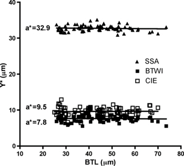
Figure 18: Thorpe's normalization of internal buccal tube width (BTWI), claw length (CIE), and distance between stylet support points (SSA) vs buccal tube length (BTL) in Paramacrobiotus tonollii. Note that all of the slopes appear very near zero, indicating the successful removal of body size effects (Bartels et al., 2011).
This data further reinforces the idea that Thorpe normalization is a strong tool for removing body size effects in samples of allometric trait measurements and is in fact more effective than the standard technique of pt-indexing.
Applications of Thorpe normalization in species delineation
As a phylum containing three classes, tardigrades are an incredibly diverse taxon. In fact, there are over 1200 known tardigrade species spanning a vast array of environments (Weronika & Lukasz, 2016). As a result, it is extremely difficult for researchers to accurately classify specimens or differentiate species without an understanding of traits independent of body size.
Thorpe normalization, as the current most effective form of body size elimination in the study of allometric traits in tardigrades, is able to help resolve this issue by providing a means of calculating trait value independent of body size, and therefore differentiating between or identifying species via these independent values.
For instance, the buccal tube is shown to be wider in certain tardigrade species, but buccal tube width also increases with body length. With the use of Thorpe normalization, the effects of body size can be removed, allowing differentiation of species based solely on the trait under consideration (namely buccal tube width). In particular, Thorpe normalization paired with discriminant analysis allowed researchers to classify specimens as belonging to either M. recens or M. hulefandi based on buccal tube length, as shown in Fig. 19 and 20 (Bartels et al., 2011). The study even notes that “if this analysis were carried out with pt indices, it would be impossible to know if the differences were due to size or to inherent species differences.”
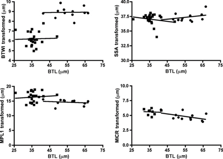
Figure 19: Thorpe normalization for internal buccal tube width (BTWI), distance between stylet support points (SSA), MPL1 (macroplacoid length), and MICR (microplacoid length) vs buccal tube length (BTL) for two species M. recens and M. hufelandi (Bartels et al., 2011).
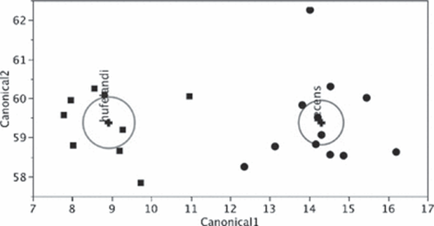
Figure 20: Discriminant analysis of M. recens and M. hufelandi using Thorpe normalization of trait measurements, allowing the differentiation of samples between the two species (Bartels et al., 2011).
Conclusion
Tardigrades demonstrate a broad array of incredible mathematical design solutions that facilitate their success in the unique environments they inhabit and in the unique behaviors they partake in, as summarized in Fig. 21. For instance, tardigrades' foraging patterns are shown to closely adhere to an algorithmic predatory model, defined by established mathematical laws, that allows them to prioritize certain prey and determine how much time to spend foraging for specific types of prey (dependent on the time and energy that must be invested as compared to the nutrient “reward”). Ultimately, following this algorithm allows them to benefit from an optimal biomass gain in all situations, regardless of variable environmental or organismal circumstances, such as prey densities or hunger levels. Moreover, tardigrade morphology has been observed to be mathematically optimized and specialized according to specific behavioral habits. For instance, the morphology of the buccal tube in particular has been demonstrated to be mathematically optimized specifically for herbivore tardigrades to consume their food most effectively.
Mathematics is essential to understanding tardigrade morphology and behavior, but it also provides the foundational steps for enabling scientists to “mimic” tardigrade solutions in biomimetic designs. For instance, the techniques of Thorpe normalization and pt-indexing allow researchers to remove body size effects from trait data and therefore more effectively compare traits between differing samples within both the tardigrade phylum and even beyond it. Mathematical modelling has even allowed tardigradologists to understand how the optimization of the buccal apparatus in different ways has allowed tardigrades to most effectively hunt specific types of prey, or to predict and model their foraging patterns.
It is only by understanding the mathematics underlying tardigrade physiology and behavior that scientists are able to take a reasoned biomimetic approach without relying on hypotheses as to the rationale behind the tardigrade's fundamental design. Ultimately, much of scientific history has involved trial and error, and exploration without full understanding. It is the mathematical understanding, paving the way for a physical, then chemical, and then biological understanding, that pushes this exploration beyond science into the realm of engineering and design.
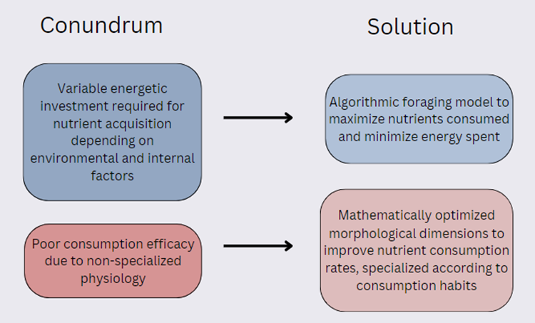
Figure 21: Diagram representing the conundrums (left) faced by the tardigrade and the solutions (right) that have been evolved to mitigate them.
References
Bartels, P.J., Nelson, D.R. and Exline, R.P. (2011), Allometry and the removal of body size effects in the morphometric analysis of tardigrades. Journal of Zoological Systematics and Evolutionary Research, 49: 17-25. https://doi.org/10.1111/j.1439-0469.2010.00593.x
Berdan, R. (2018). How to Collect and Photograph Water Bears (Tardigrades) by Robert Berdan – The Canadian Nature Photographer. https://www.canadiannaturephotographer.com/waterbears.html
Bingemer, Jana & Hohberg, Karin. (2017). An illustrated identification key to the eutardigrade species (Tardigrada, Eutardigrada) presently known from European soils. Soil Organisms. 89.
Britannica, T. Editors of Encyclopaedia (2023, October 17). tardigrade. Encyclopedia Britannica. https://www.britannica.com/animal/tardigrade
Drew Z, Bell D, Voxel size (2018). Reference article, Radiopaedia.org (Accessed on 30 Nov 2023) https://doi.org/10.53347/rID-62838
Feng, C., Wang, H., Lu, N., Chen, T., He, H., Lu, Y., & Tu, X. M. (2014). Log-transformation and its implications for data analysis. Shanghai archives of psychiatry, 26(2), 105–109. https://doi.org/10.3969/j.issn.1002-0829.2014.02.009
Gribkova, E. D., Lee, C. A., Brown, J. W., Cui, J., Liu, Y., Norekian, T., & Gillette, R. (2023). A common modular design of nervous systems originating in soft-bodied invertebrates. Frontiers in physiology, 14.
Gross, V., Müller, M., Hehn, L. et al. X-ray imaging of a water bear offers a new look at tardigrade internal anatomy. Zoological Lett 5, 14 (2019). https://doi.org/10.1186/s40851-019-0130-6
Guidetti, R., Bertolani, R., & Rebecchi, L. (2013). Comparative analysis of the tardigrade feeding apparatus: adaptive convergence and evolutionary pattern of the piercing stylet system. Journal of Limnology, 72, 24-35.
Hohberg, K., & Traunspurger, W. (2009). Foraging theory and partial consumption in a tardigrade–nematode system. Behavioral Ecology, 20(4), 884-890.
Hohberg, K., Traunspurger, W., 2005. Predator-prey interaction in soil food web : functional response, size-dependent foraging efficiency, and the influence of soil texture. Biol. Fertil. Soils 41, 419–427. https://doi.org/10.1007/s00374-005-0852- 9.
Ingemer, Jana & Hohberg, Karin. (2017). An illustrated identification key to the eutardigrade species (Tardigrada, Eutardigrada) presently known from European soils. Soil
Jeschke, J. M., & Hohberg, K. (2008). Predicting and testing functional responses: an example from a tardigrade–nematode system. Basic and Applied Ecology, 9(2), 145-151.
Jönsson, K. Ingemar, et al. Tardigrades Survive Exposure to Space in Low Earth Orbit, current biology, 9 Sept. 2008, doi.org/10.1016/j.cub.2008.06.048.
Lleonart J, Salat J, Torres GJ (2000, July 7). Removing allometric effects of body size in morphological analysis. J Theor Biol;205(1):85-93. doi: 10.1006/jtbi.2000.2043. PMID: 10860702.
Macdonald, H. (2004) Geologic Puzzles: Morrison Formation, Starting Point. Retrieved Sept 9, 2004, from http://serc.carleton.edu/introgeo/interactive/examples/morrisonpuzzle.html
Manly, B., Miller, P., & Cook, L. (1972). Analysis of a selective predation experiment. The American Naturalist, 106(952), 719-736.
Mayer, G., Kauschke, S., Rüdiger, J., & Stevenson, P. A. (2013). Neural markers reveal a one-segmented head in tardigrades (water bears). Plos one, 8(3), e59090.
Nelson D. R. (2002). Current status of the tardigrada: evolution and ecology. Integrative and comparative biology, 42(3), 652–659. https://doi.org/10.1093/icb/42.3.652
Peluffo, J. R., Rocha, A. M., & de Peluffo, M. M. (2007). Species diversity and morphometrics of tardigrades in a medium–size city in the Neotropical Region: Santa Rosa (La Pampa, Argentina). Animal Biodiversity and Conservation, 30(1), 43-51.
Pilato, G. (1981). Analisi di nuovi caratteri nello studio degli Eutardigradi. Animalia, 8.
Reist, J. D. (1985). An empirical evaluation of several univariate methods that adjust for size variation in morphometric data. Canadian Journal of Zoology, 63(6), 1429-1439.
Reyes, E., Nuñez, P., & Vázquez, R. (2023). Tardigrades, Thousand Environments to Survive. Revista Mexicana de Astronomia y Astrofisica Conference Series.
Roszkowska, M., Bartels, P. J., Gołdyn, B., Ciobanu, D. A., Fontoura, P., Michalczyk, Ł., Nelson, D. R., Ostrowska, M., Moreno-Talamantes, A., & Kaczmarek, Ł. (2016). Is the gut content of Milnesium (Eutardigrada) related to buccal tube size? Zoological Journal of the Linnean Society, 178(4), 794-803.
Shingleton, A. (2010) Allometry: The Study of Biological Scaling. Nature Education Knowledge 3(10):2
Stephens, D. W., & Krebs, J. R. (1986). Foraging theory (Vol. 1). Princeton university press.
ter Braak, C.J.F., Sˇmilauer, P., 2012. Canoco Reference Manual and User's Guide: Software for Ordination, Version 5.0. Microcomputer power, Ithaca USA
Surette, F. 2014. “Hypsibius dujardini” (On-line), Animal Diversity Web. Accessed December 01, 2023 at https://animaldiversity.org/accounts/Hypsibius_dujardini/
Tůmová, M., Stec, D., Michalczyk, Ł., & Devetter, M. (2021). Buccal tube dimensions and prey preferences in predatory tardigrades. Science direct. https://doi.org/10.1016/j.apsoil.2021.104303 Weronika, E., & Łukasz, K. (2017). Tardigrades in Space Research – Past and Future. Origins of life and evolution of the biosphere : the journal of the International Society for the Study of the Origin of Life, 47(4), 545–553. https://doi.org/10.1007/s11084-016-9522-1
[1] rA2 here stands for the same defined ratio, but in the form A2:A1.
[2] s is thus described “if a man is satiated with 10 potatoes in his stomach, then s = 0.1” (Jeschke & Hohberg, 2008).
[3] h = 0 meaning no hunger at all, and h = 1 referring to a maximal hunger level.