Population Dynamics for Mutualistic Relationships

Beth Cushnie, Dorothy Ma, Anh Ngo, Tanoulu Li

Abstract

Mathematics is increasingly present in various disciplines and especially in biology. Modeling in biology began to be used in population dynamics to model the growth of populations and the multiple interactions that may exist between them. There are many different types of models that can be constructed, with various levels of complexity, for various situations. Which model one chooses depends on what they would like to study. In this paper, the general equations for mutualistic population dynamics are considered, as well as specific cases. Different methods to model bee populations and are compared and explained. To understand the difficulty of applying mathematics in nature, we study the relationship between yucca plants and yucca moths. Finally, to contrast and get a better understanding of the mathematical relation of interspecies interactions, we explored the population dynamics of parasitic relationships.

Introduction

Ecological systems are established and maintained by the species that coexist within it. Most, if not all, species in the ecosystem interact between one another, either directly or indirectly. This paper will examine mutualistic and parasitic relationships between species and what that means in terms of their population dynamics. Mutualism occurs when species interact in a way that is mutually beneficial. Parasitism describes a relationship that is beneficial for one of the species and detrimental to another. The populations of species are influenced by other species they interact with, and in turn, form symbiotic relationships with. When the size or density of one involved population changes, the population of the other species in the relationship is affected (Holland, 2012).

The population of a species is primarily influenced by density-independent and density-dependent factors of their environment (Holland, 2012). Density-independent factors affect a given population regardless of its density, such as weather events (Holland, 2012); a severe rainstorm will affect an ant colony regardless of if the ant colony has 10 ants or 10 000 ants. On the other hand, density-dependent factors change relative to the density of the population, such as available space, food, and other limited resources (Holland, 2012).  

In population dynamics, an important density-dependent factor is the interspecific interactions, also known as consumer-resource (C-R) interactions (Holland & DeAngelis, 2010). C-R interactions are relations where the species involved can provide for and consume the resources provided by the other species and vice versa (Holland & DeAngelis, 2010). Nearly all mutualistic relationships follow one of three C-R interactions: bi-directional, uni-directional, or indirect mutualism (Holland & DeAngelis, 2010). Bi-directional relationships involve two species who both act as both the consumer and resource for the other species (Holland & DeAngelis, 2010). Meanwhile, uni-directional relationships involve one species that acts solely as the resource while the other acts solely as the consumer (Holland & DeAngelis, 2010). The consumer, while not directly supplying a resource, will provide a non-trophic service, such as seed dispersal or protection from other species, maintaining the mutually beneficial relationship (Holland & DeAngelis, 2010). Indirect mutualism involves a third species, which mediates the relationship, often acting as a consumer or resource for one or both involved species (Holland & DeAngelis, 2010). Functional responses can be used to model the population of one species as a function of its mutualist species. The relationship between the two species is not as clear for indirect mutualism and will therefore not be expanded upon in this paper.

Bi-directional and Uni-directional Mutualism Models

In mutualism, the population of one species is dependent on the density of its mutualist species and can thus be written as in relation to the latter species. Different types of mutualism involve different relationships, such as obligate and facultative. Obligate relationships are when species are entirely codependent, while facultative means that the species can exist separate from the mutualist partner. Holland et al. (2002) proposed the following model for obligate mutualistic relationships:

{dN_2\over dt} = B_nN_2 - dN_2 - gN_2^2

where N₂ is the population size of species 2, B_n is the net effect of the mutualistic species for species 2, d is the mortality rate, and g is the rate of self-limitation. In their model, the net effect B_n of the mutualistic relationship is measured by the gross benefit from the relationship minus the cost of being in the relationship, such as supplying resources, which is generally the functional response f(N₁,N₂). Some examples of B_n as determined by non-linear gross benefit and cost functions are shown in Figure 1.

This model is for obligate relationships only, as seen that the only positive value comes from the first term; if the mutual species is absent (B_n = 0), the population will strictly decrease.

{dN_i\over dt} = N_i[r_i+c_if_i(R_j)-q_ig_i(R_i) - d_iN_i]

This model can be broken down into a more generally applicable model. This second model, proposed by Holland and DeAngelis (2010), shows the differences in bi-directional and uni-directional as well as obligate and facultative mutualistic relationships:

The first and last terms are the population growth rate independent of mutualism, which in fact represent a logistic growth. r_i – d_iN_i shows that when N_i approaches 0, the growth rate is nearly r_i, and decreases by d_i with an increasing population.

{dN_i\over dt} = N_i[c_if_i(Rj)-q_ig_i(R_i)-d_iN_i]

In an obligate relationship, the r_i term is set to 0, to indicate that the population will not grow in the absence of the mutual species:

R_j is a function of both population sizes (N_i, N_j) that represents the gross benefit of the relationship for species j. R_i is a function of both population sizes representing the cost of the relationship for species i. The two together is equivalent to the net effect of the mutual relationship on the population growth rate of species i. The variables c, f, q, and g are coefficients that convert R_j and R_i into numerical values. This equation models a bi-directional relationship.

It can model a uni-directional relationship by removing the third term q_ig_i(R_i) such that the species i is not contributing a resource to the relationship while consuming the benefits.

{dN_i\over dt} = N_i [r_i + c_if_i(R_j)-d_iN_i]

Different Ways to Model the Population of Bees

Bees are an incredibly vital part of the ecosystem, but due to climate change, habitat destruction, and the widespread use of pesticides, populations are dwindling. Because of this, their populations have become a prevalent subject for researchers, and a common way they analyze them is through population dynamics. There are many different proposed models, all with slightly different factors and varying levels of complexity, but they all try to provide a tool to understand the population of bees, to help find a solution to their decreasing numbers. Of course, one of the most important factors is the food supply. Bees and flowers have one of the most well-known mutualistic relationships, with bees relying on flowers for food, and flowers relying on bees for reproduction. Their populations are highly linked, but generally mathematical models focus on the bees, with the flowers being a related factor.

Khoury et al. (2011) focused on creating a simple model to help predict colony collapse disorder (CCD), where the entire colony of bees dies rapidly. While most of the reasons for declining bee populations are well known, these extreme cases of CCD are not well understood.

Understanding CCD is the first step to preventing it from happening. Khoury et al. (2011) worked off the hypothesis that colony failure occurs when the death rate of bees in the colony is unsustainable. While this is not particularly groundbreaking, they focused specifically on how forager bees dying causes young hive bees to become foragers too early. Forager bees have a much higher death rate than hive bees, so it decreases the lifespan of the bee, and decreases their amount of time spent in the nest. Overall, it messes up the cycle of the nest, and compounds the problem.

Fig. 2 is a representation of the bee colony created by Khoury et al. (2011) and was used to visualize the changing populations.  Baby bees become hive bees, who become foragers. The population of each group depends on the population of the others; if there are too few foragers, more hive bees will become foragers. If there are too few hive bees looking after the nest, foragers can convert back to hive bees. The need for foragers generally overrides this, but it does work to inhibit the number of foragers. The number of brood depend on the number of adult bees. Foragers have a higher rate of death. One thing to note is that this model assumes that the death rate of hive bees is negligible, and does not consider the impact of brood diseases. However, this model is straightforward and easy to understand.

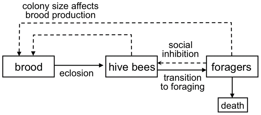
Khoury et al. (2011) represented this population using the following equations:

Rate of change of hive bee numbers:

{dH\over dt}=E(H,F)-HR(H,F)

Rate of change of forager numbers:

{dF\over dt}=HR(H,F)-mF

Number of eclosions (hatchings):

E(H,F)=L({N\over w+N})=L({H+F\over w+H+F})

Recruitment rate function (number of hive bees turning into foragers):

 R(H,F)=α-σ({F\over H+F})

H is the number of hive bees, and F is the number of foragers. N is the total number of adult bees (H+F=N). t is time, in days. L is the queen’s laying rate. w is a constant, and determines the rate at which E(H,F) approaches L as N gets large. Alpha is the maximum rate that hive bees will become foragers when there are no foragers present in the colony, and the second term of that equation represents social inhibition and how the presence of foragers reduces the rate of recruitment of hive bees to foragers.

Using standard linear stability analysis and phase plane analysis, they found the globally stable stead state (H₀,F₀):

F_0={L\over m}-w({J\over J+1}),    H_0={1\over J} F_0

where

J = \frac{1}2{} ((\frac{\alpha}{m}-\frac{\sigma}{m}-1)) + \sqrt{(\frac{\alpha}{m}-\frac{\sigma}{m}-1)^{2} + \frac{4\alpha}{m}}

when

m < \frac{L}{2w} ((\frac{\alpha}{m}-\frac{\sigma}{m}-1) +\sqrt{(\frac{a}{m}-\frac{\sigma}{m}-1)^2 + \frac{4\alpha}{m}}) = \frac{L}w{J}\, and\, \alpha-\frac{L}{w} > 0 

Khoury et al. (2011) created a phase diagram to better visualize the results (Fig. 3). Fig. 3.a is when m is less than (L/w)J. There is an equilibrium, and the population can sustain itself. Fig. 3.bis when m is greater than (L/w)J. No matter what your population is, or what any of the other factors are, the population will collapse to zero.

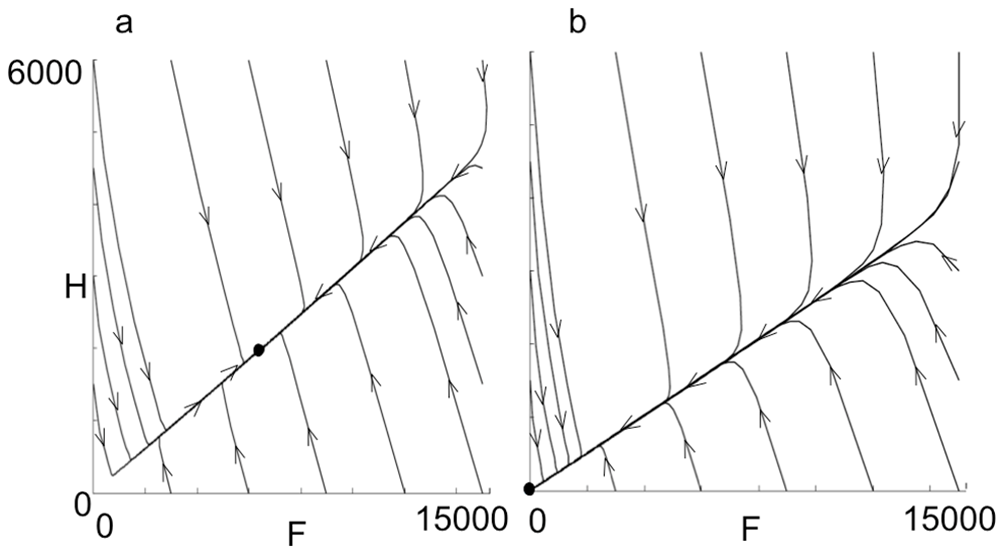
Because this is a simple model, there is a limited amount of analysis one can do with it. However, it is excellent for representing how forager death rate has such a strong influence on the population size. If the death rate of foragers is too high, the population quickly disappears, no matter what the other factors are. This could help explain colony failure.

Khoury et al. made another model in 2013. This model expands upon their first equation, but incorporates food supply as well. A food shortage causes more hive bees to become foragers, and the effects of this were discussed above, and it diminishes the size of the brood. Overall, the situation can be visualized in Fig. 4.

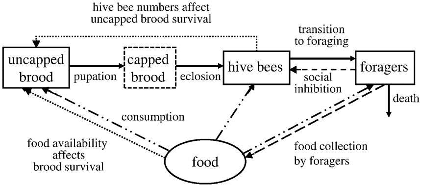
This model requires 9 different equations to properly describe it. Analyzing it reveals the relationship between food availability and population. When there is a low death rate, the food availability determines the population. However, as the death rate increases, the relationship becomes much more complex, and the equilibrium point depends on all the variables. Different outcomes include a stable population with an excess of food stores, to a stable population with limited food stores, to zero population with residual food stores. This more complex model can be used for more detailed analysis of bee populations, and more in-depth understanding of the different factors and their effects.

Models can be much, much more complicated though. Banks et al. (2017) developed a delay differential equation to model the population of bees. In DDEs, the derivative of the unknown function is given in terms of the values of the function at previous times. This allowed their model to incorporate specific time intervals for between important events, such as the laying of the eggs, and the emergence of the bee. Their model specifically focused on the environment and how the use of toxins affected the population, but included information on colony establishment, mortality, colony growth, reproduction, and queen hibernation.

This model included 7 variables, 4 timelines, 22 parameters, and came to 22 different equations. This produced a much more nuanced and accurate model for bee population compared to the ones developed by Khoury et al. (2011, 2013), but is much harder to work with and understand. Their model did not produce any surprising results—for example, low food supplies and high death rates caused the colony to collapse, just as previous models had—but it provided a more rigorous mathematical explanation, and can be used to model different situations.

Mutualism between Yucca and Yucca moths

The plant and its pollinator necessarily depend on each other. A female yucca moth collects pollen from yucca flowers, flies to another group of flowers, and lays its eggs at the pistil’s base of a newly opened flower (Riley, 1892). After laying her eggs, the female moth rises to the top of the pistil and then places the pollen it previously collected on the stigma of the flower (Riley, 1892). The moth larvae hatch, then feed on the yucca seeds (Riley, 1892). Thus, the moth pollinates the plant and feeds on its seeds.

In a situation where there is no cost for the plant, the moth would carry the pollen but would not destroy the seeds of the plants (Riley, 1892). In a no-cost situation for the moth, the moth would produce as many larvae as possible and consume several plant seeds. In reality, an evolving compromise has taken place (Riley, 1892). This is because the moth usually only lays a few eggs per flower and the plant tolerates the loss of some of its seeds. The yucca has a defense mechanism that participates in preserving this compromise: if a moth lays too many eggs on the flowers, the plant can selectively cause the seeds of this flower to “abort” (Riley, 1892). It thus eliminates the eggs.

This relationship can be illustrated graphically in Figure 5 below.

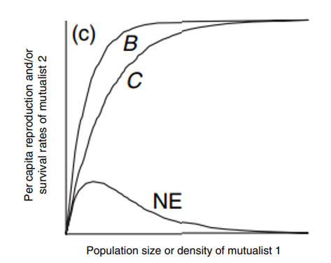
The moth larvae hatch then consume seeds. Line B in the figure illustrates that the seed production increases during moth pollination and decreases when larvae feed on seeds (Holland & Bronstein, 2008). Therefore, the seed production depends on the yucca moths: a low moth density is followed by a low plant reproduction (Holland & Bronstein, 2008).

However, a high moth density does not result in an increasing non-stop plant reproduction. Indeed, when all the flowers are pollinated, even if the moth density keeps increasing, the seed production and benefit stay stagnant, as shown by line B (Holland & Bronstein, 2008).

The cost follows the same behavior as the benefit pattern, as shown by line C. The costs of seed consumption represent the oviposition’s rate (Holland & Bronstein, 2008). As the moth density increases, the oviposition’s rate also increases (Holland & Bronstein, 2008). However, we arrive at one point, even if the moth density keeps rising, the seed consumption stays the same because all the seeds are eaten (Holland & Bronstein, 2008).

From that, we have the net effect of plant reproduction measured by the final quantity of seed production, which is determined by NE = B – C. Thus, the net effect is a unimodal function of moth density.

The real representation of the relationship

In July and August 1980, Addicott did research on 690 mature yuccas fruits from eight species, and all of them are pollinated by T. yuccasella. He examined each of them. He counted the left-over seeds and classified them based on whether they were eaten or not and viable or not (Fig. 6). He also counted the moth larvae (Fig. 7).

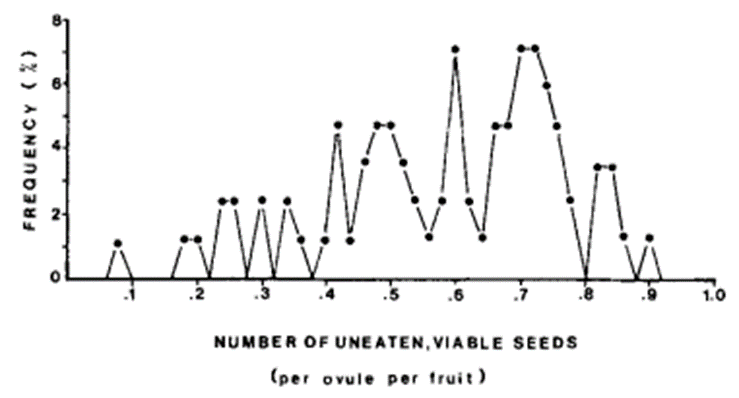
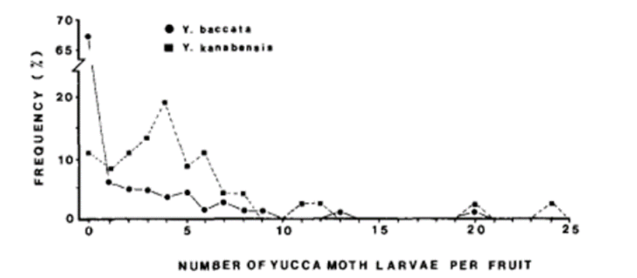
Addicott (1986) found out that only 0.0-13.6% of viable seeds were consumed by yucca moth larvae per fruit. Thus, the ratio of costs to benefits was between 0% and 30%. This means that this relationship is in favor of yuccas plants. The moths can only benefit for a maximum 30%. Addicott (1986) later compared his research results with research involving figs and gid wasps done by Janzen (1979). The costs values indeed are lower and more variable in the mutualism relationship between figs and fig wasps.

The costs’ variation makes it challenging to present graphically this mutualism between yucca and yucca moths (Addicott, 1986). Indeed, to understand the dynamics of population and the evolution of mutualism, controlling the costs, benefits, and net benefits is necessary. However, it is not easy to satisfy these criteria. Indeed, we cannot compare costs and benefits since they do not have the same biological currency (Southwick, 1984). The second problem is that we could never control the variables because the environment affects the species’ interdependence (Addicott, 1986).

The Mathematical Models of Population Dynamics between Parasitoids and their Hosts

Parasitoids are insects that are born and developed on or in the tissues of other arthropods. With the growth of the larvae of the parasitoids, the host will eventually be killed (Hassell & Waage, 1984). The population dynamics is constantly changed in the host-parasitoids interaction (Singh & Emerick, 2020). To identify the change in population in the parasitoid-host relationship, scientists developed many mathematical models. This part of the essay will introduce two classic mathematical models to show how to model the population dynamics approximately.

Nicholson–Bailey Model

Parasitoids lay their eggs into the hosts, and they grow in a host as parasites. However, they will become predators, as introduced above, leading to the death of their host (Hassell & Waage, 1984). Therefore, the variables, the number of birth of parasitoids and the number of surviving hosts, will be vitally important to analyze the population dynamics. The Nicholson-Bailey model is a basic and classic discrete-time mathematical model describing the population dynamics in parasitoids-host interaction (Jervis & Kidd, 1986; Logan & Wolesensky, 2009). The model is a coupled set of differential equations given by Logan & Wolesensky (2009):

H_{(t+1)}=d(H_t ) H_t f(H_t,P_t)

P_{(t+1)}=c(H_t )(1-f(H_t,P_t ))

Or equivalently,

H_{(t+1)}=RH_te^{(-aP_t )}

Where t is the year, H and P are the host and parasitoid populations at the year, R represents the number of surviving unparasitized hosts, a is a constant that approximates the probability that the host are not parasitized after meeting the parasitoids, and the parameter c is the number of larvae born in the hosts.

Lotka–Volterra Model

In contrast to the discrete-time model, Nicholson-Bailey model, Lotka-Volterra Model, known as predator-prey equations, is a continuous-time model of non-linear differential equations, describing the ecological system of predator and preys (Gotelli, 2018; Krivan, 1997). Because the host-parasitoid relationship is a special kind of prey-predator relationship, the Lotka-Volterra Model can also approximate the population dynamics of host-parasitoid interactions with time (Gotelli, 2018; Krivan, 1997).

The equations are (Gotelli, 2018; Odum, 1963):

{dx\over dt}=x(A-By)

{dy\over dt}=y(-C-Dx)

Where x is the number of parasitoids while y is the number of hosts, t is continuously time, dx/ dy and dy/dt illustrate the rate of change of the population of parasitoids and hosts throughout time, and the parameters A,B,C and D illustrate the host-parasitoid interaction.

Limitations of the two models

However, the two models above are too simple to simulate the complex parasitoid-host systems. Both two models make many assumptions, and a very large number of biological and non-biological factors are not considered (Gotelli, 2018; Logan & Wolesensky, 2009; Krivan, 1997). For example, both are limited to being applied to only two species and consider food resources ultimate (Gotelli, 2018; Logan & Wolesensky, 2009; Odum, 1963). They do not consider the factors of the intraspecific competition within the two species and the migration of species (Kopp & Gabriel, 2006; Rafikov et al., 2008). Therefore, ecologists and mathematicians focus on improving the models to more precisely match the approximation with the real-world ecological condition.

Here is an example in more detail. Host-feeding is an excellent and exciting factor that may be considered to improve the mathematical model of parasitoids. Many species of parasitoids are known to use the hosts for reproductive purposes and short-term food sources (Chan & Godfray, 1993; Lewis et al., 1998). The term “host-feeding” is defined as using host material as food by adult female parasitoids (Jervis & Kidd, 1986). Using more hosts as food, the survival rate and lifespan of the parasitoids will increase, though the number of available hosts for laying and incubating eggs will decrease (Chan & Godfray; Krivan, 1997). Therefore, the phenomenon of host-feedings may affect the population dynamics approximation if using the models above because it is an extra factor that these models do not consider. To improve the model, we need research on the strategies developed by parasitoids on balancing the two uses of their hosts, oviposition vs. nutritional sources. (Chan & Godfray).

Conclusion

Population dynamics is an incredibly complicated and vast field. Populations are constantly changing, and are affected by a multitude of different factors, and fitting it into a neat mathematical equation is almost impossible. This problem is compounded when dealing with mutualistic relationships, as it is another factor that a population heavily depends on. That being said, researchers try their best, as having these mathematical models is extremely useful for understand and articulating the relationships between species, and populations in general. They are a vital tool for understanding a population, and as we learn more about how different species interact, and how they grow, our models can only get more accurate.

References

Addicott, J. F. (1986). Variation in the costs and benefits of mutualism: the interaction between yuccas and yucca moths. Oecologia, 70(4), 486-494. https://doi.org/10.1007/BF00379893

Banks, H. T., Banks, J. E., Bommarco, R., Laubmeier, A. N., Myers, N. J., Rundlöf, M., & Tillman, K. (2017). Modeling bumble bee population dynamics with delay differential equations. Ecological Modelling, 351, 14-23. https://doi.org/https://doi.org/10.1016/j.ecolmodel.2017.02.011

Chan, M. S., & Godfray, H. C. J. (1993). Host-feeding strategies of parasitoid wasps. Evolutionary Ecology, 7(6), 593-604. https://doi.org/10.1007/BF01237823

Gotelli, N. J. (2008). A Primer of Ecology (Fourth ed.). Sinauer Associates.

Hassell, M. P., & Waage, J. K. (1984). Host-Parasitoid Population Interactions. Annual Review of Entomology, 29(1), 89-114. https://doi.org/10.1146/annurev.en.29.010184.000513

Holland, N. J. (2012). Population Dynamics of Mutualism. Nature Education Knowledge, 3(10). https://www.nature.com/scitable/knowledge/library/population-dynamics-of-mutualism-61656069/

Holland, N. J., & Bronstein, J. L. (2008). Mutualism. In S. E. Jørgensen & B. D. Fath (Eds.), Encyclopedia of Ecology (pp. 2485-2491). Academic Press. https://doi.org/https://doi.org/10.1016/B978-008045405-4.00673-X

Holland, N. J., & DeAngelis, D. L. (2010). A consumer–resource approach to the density-dependent population dynamics of mutualism. Ecology, 91(5), 1286-1295. https://doi.org/https://doi.org/10.1890/09-1163.1

Holland, N. J., DeAngelis, D. L., & Bronstein, J. L. (2002). Population Dynamics and Mutualism: Functional Responses of Benefits and Costs. The American Naturalist, 159(3), 231-244. https://doi.org/10.1086/338510

Janzen, D. H. (1979). How Many Babies Do Figs Pay for Babies? Biotropica, 11(1), 48-50. https://doi.org/10.2307/2388172

Jervis, M. A., & Kidd, N. A. (1986). Host-feeding strategies in hymenopteran parasitoids. . Biological Reviews, 61(4), 395-434. https://doi.org/https://doi.org/10.1111/j.1469-185X.1986.tb00660.x

Khoury, D. S., Barron, A. B., & Myerscough, M. R. (2013). Modelling Food and Population Dynamics in Honey Bee Colonies. PLOS ONE, 8(5), e59084. https://doi.org/10.1371/journal.pone.0059084

Khoury, D. S., Myerscough, M. R., & Barron, A. B. (2011). A Quantitative Model of Honey Bee Colony Population Dynamics. PLOS ONE, 6(4), e18491. https://doi.org/10.1371/journal.pone.0018491

Kopp, M., & Gabriel, W. (2006). The dynamic effects of an inducible defense in the Nicholson–Bailey model. Theoretical Population Biology, 70(1), 43-55. https://doi.org/https://doi.org/10.1016/j.tpb.2005.11.002

Krivan, V. (1997). Dynamical consequences of optimal host feeding on host-parasitoid population dynamics. Bulletin of Mathematical Biology, 59(5), 809-831. https://doi.org/https://doi.org/10.1016/S0092-8240(97)00029-3

Lewis, W. J., Stapel, J. O., Cortesero, A. M., & Takasu, K. (1998). Understanding How Parasitoids Balance Food and Host Needs: Importance to Biological Control. Biological Control, 11(2), 175-183. https://doi.org/https://doi.org/10.1006/bcon.1997.0588

Logan, J. D., & Wolesensky, W. (2009). Mathematical Methods in Biology. Wiley.

Odum, E. P. (1963). Ecology. Holt, Rinehart and Winston.

Rafikov, M., Balthazar, J. M., & von Bremen, H. F. (2008). Mathematical modeling and control of population systems: Applications in biological pest control. Applied Mathematics and Computation, 200(2), 557-573. https://doi.org/https://doi.org/10.1016/j.amc.2007.11.036

Riley, C. V. (1892). The Yucca Moth and Yucca Pollination. Missouri Botanical Garden Annual Report, 1892, 99-158. https://doi.org/10.2307/2992075

Singh, A., & Emerick, B. (2021). Generalized stability conditions for host–parasitoid population dynamics: Implications for biological control. Ecological Modelling, 456, 109656. https://doi.org/https://doi.org/10.1016/j.ecolmodel.2021.109656

Southwick, E. E. (1984). Photosynthate Allocation to Floral Nectar: A Neglected Energy Investment. Ecology, 65(6), 1775-1779. https://doi.org/10.2307/1937773