A Mathematical Analysis of Animal Horns
Lily Trestan, Rachel Jung, Toufic Jrab, Victor Novakov
Abstract
The following essay examines the application of mathematics to biological structures, in particular animal horns. It begins by exploring the evolutionary reasons for ornamental appendages among horned animals. Mathematical computations reveal a relationship between ornament size and “honest advertisement” due to a high cost of having such large appendages. Furthermore, horn symmetry is antisymmetric rather than fluctuating or directional symmetry. This form of symmetry generates a bimodal distribution and reflects poor developmental conditions among the population. The middle section of the paper highlights the shapes and sequences revealed through the horns of certain animal species. Animals with helical shaped horns display bilateral symmetry which can be homonymous or heteronymous depending on their enantiomeric arrangements. Biological structures such as horns commonly form advantageous structures like logarithmic spirals and are linked to specific commonly occurring numbers like the golden ratio, and the Fibonacci sequence. However, other models such as the Power Cascade may be more accurate in quantifying such appendages. Computationally, methods for analyzing animal horns are examined in the final sections of the paper, which demonstrate how these models and computations are integrated into engineering today. Finally, through various modeling simulation techniques, the key furrow regions of the primordium of the beetle horn can be linked to the final 3D shape of the fully grown beetle horn.
Introduction
The wild is an unpredictable and incalculable environment; however, after years of collecting data and recording evolutionary change over a large population of animals, clear patterns and relationships in biological properties arise. When studying any aspect of nature, statistical analysis and mathematical models are integral tools in understanding the shape and complex nature of these structures, and animal horns are no different. This paper explores the underlying mathematics of evolutionary and environmental effects on horns. Namely, this paper dives into quantifying the evolutionary effects on horn design and symmetry, as well as investigate the mathematical models of the shapes that horns typically take on, such as helices, the logarithmic spiral, and power cascades, in order to understand how these impressive structures occur. Once the fundamentals of mathematics in nature are established, the applications of these computational models and theories are discussed, and the significance of these arithmetic techniques becomes apparent.
Evolutionary and environmental influence on horns
Quantifying the evolution of ornamental design
The animal kingdom is full of animals with impressive physical features such as the intricate and colorful feathers of the peacock and the spiraled horns of antelopes. This is not a random phenomenon. In fact, scientists continue to try and quantify these patterns of evolution. One explanation comes when looking at the evolution of male animals as they combat the tension between natural selection and sexual selection which groups them into one of two categories: animals with distinct and costly ornamentation which can increase sexual capital or those with less costly subtle ornaments.
For many animals it is obvious why natural selection selects certain characteristics. Male peacocks use their feathers and dance to attract females, and most Bovidae and cervid horns and antlers are useful in contests. However, not all appendages are beneficial, and the horned beetle is the perfect example of this. The large size of their horns handicaps the animal, yet it is still selected for. Zehavi’s handicap principle, from 1975, provides an explanation for this phenomenon that is still relevant today (“Study Explains Evolution Phenomenon That Puzzled Darwin”). Essentially, ornaments advertise individual quality and thus it must be physically taxing and costly on the individual to ensure honest advertisement, which makes the mating process more efficient (Clifton et al., 2016).
Charles Darwin was the first to formulate the theory that both natural and sexual selection play a role in evolution. Natural selection is based on an individual’s ability to survive in their environment. Sexual selection is based on an individual’s ability to find a good mate and reproduce. Darwin puts forth that a female’s preference for over-the-top male features is the evolutionary drive for ornamentation; however, he was not able to deduce why females prefer males, which are often handicapped by their appendages (Clifton et al., 2016). Such as the case of the horned beetle, which is illustrated in Figure 1.

Fig. 1. Dimorphic ornament example of two dung beetles with different horn lengths (Clifton et al., 2016).
To expand on the previous hypothesis, an ornament that has negative implications on an individual, overtime, ensures that only the most fit individuals can invest in them. Thus, females can trust that their mate is of quality despite their disabilities.
In a study by M. Clifton et al. 2016, researchers developed a mathematical model for the handicap principle, which is independent of a particular phenotype and allows for the scenario in which there is an optimal distribution of strategies that can emerge from a population.
To start, their model incorporates two components:
- Natural Selection: The individual cost of ornamentation and its effect on survival.
- Sexual Selection: The reproductive benefit of having large ornamentation with the opposite sex.
And finally, they assume that animals that are in identical form and health are forced by these two factors, to either develop large ornaments or small ones. The model relies on the idea of reproductive potential, F. And, over periods of time, evolution selects for animals with a higher reproductive potential. Ornamental size provides some value in survival and protection against predation; therefore, there is likely an optimal size in which the benefits outweigh the costs. The study adopted a quadratic single peak function with the following formula:
\begin{equation}
\phi^{ind}=a(a_{opt}-a)
\end{equation}φind = individual reproductive potential
aopt = optimal ornament size
Optimal ornament size is calculated with the following formula:
\begin{equation}
a_{opt}=a_{opt}(h)
\end{equation}
The intrinsic health, h, of the individual signifies that the healthier the individual, the more it can afford the ornament size. When the ornament size is compared with factors such as time, total potential and individual potential, the following graphs, as seen in Figure 2 are produced:
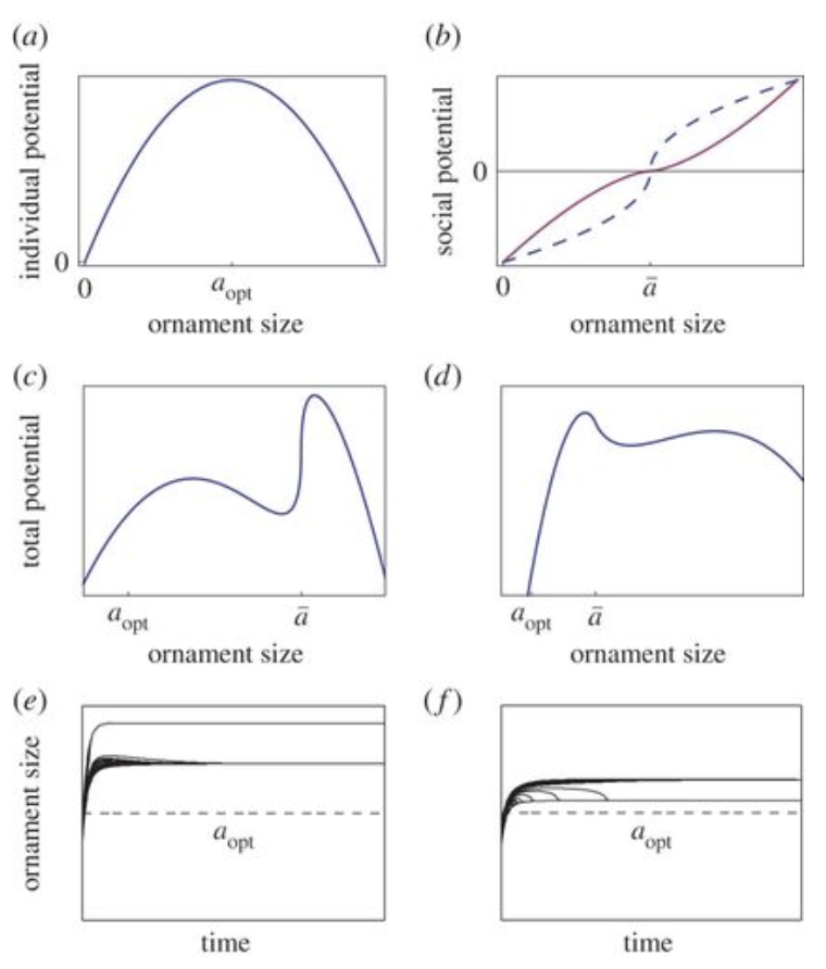
Fig. 2. Graphical analysis of ornament size as a function of individual potential (a), social potential (b), total potential (c&d). (e & f) graph the variation of ornament size as a function of time (Clifton et al., 2016).
As seen above, most graphs follow a similar trend in which individual and total potential begin to increase with size, however after a peak their relationships become inverted.
The social reproductive potential, F, represents the competition amongst same sex animals during mating. The study decided to quantify social productive power by the power of the difference between male ornament size and the entire herd average ornament size (see Eq. 3).
\begin{equation}
\phi^{soc}=sgn(a-\bar a)\lvert a-\bar a\rvert^\gamma
\end{equation}
g= “female choice” parameter
sgn= sign function
ā = average ornament size
Finally, the weighted average of reproductive potential is taken:
\begin{equation}
\phi =s\phi^{soc}+(1-s)\phi^{ind}
\end{equation}
s = relative importance of competitive social effects versus individuals’ effects (sexual selection versus natural selection)
The following formula describes how the distributions of ornament size amongst a given population changes over time due to the selection process. Because evolution optimizes reproductive potential at a proportional rate to marginalized benefits of ornamentation, ornament size expressed by:
\begin{equation}
\frac{da}{dt}=\frac{c\partial \phi}{\partial a}
\end{equation}
c = time-scaling parameter (c > 0)
When the formula is expanded by substituting the partial derivative of reproductive and social potential, and ornament size with Equations (4) and (5), the final mathematical model is as follows:
\begin{equation}
\frac{da}{dt}=c\left[s\gamma\left(\left(1-\left(\frac{1}{N}\right)\right)\lvert a-\bar a\rvert^{\gamma-1}+2(a_{opt}-a)\right)\right]
\end{equation}
N = population size
This leads to the answer reached in the study by Clifton et al. 2016 that ornament size signifies desired mate quality in the perspective of females. This is assuming that accurate derivations found in the study generally follow this relationship. The above model is based on the idea that individuals fall into one of two morph categories, which both include ornament sizes that are too large for the individual, reducing the population’s survival potential. Nonetheless, these costly appendages still prevail, supporting the idea that the evolutionary benefits of ‘honest advertising’ are greater than their costs (Clifton et al., 2016).
Horn asymmetry
Classifying asymmetry among horned animals
Any type of asymmetry will involve some form of variance from the standard or common trait. Among those is the asymmetry in the distribution of a key characteristic in a local community relative to the wider outer populations, and this presents an opportunity to observe the asymmetry of keystone adaptations such as horns between communities as a sign of external “noise” or disturbance. In fact, there are several types of asymmetries which allow researchers to describe a population and explain variances in their appearances. Fluctuating asymmetry, FA, describes small, non-directional deviations from perfect symmetry and is the result of developmental noise. This is when a phenotype varies amongst individuals with the same genotypes and environmental conditions (Mahé et al., 2021). Directional asymmetry, (DA) is a population-level difference that deviates from bilateral symmetry (Parés Casanova & Kucherova, 2013). DA depends on genotype and environmental influence (Mahé et al., 2021). Finally, antisymmetry, AS, is when a deviation favors one side in a population. This generates a bimodal distribution with zero mean (Mahé et al., 2021).
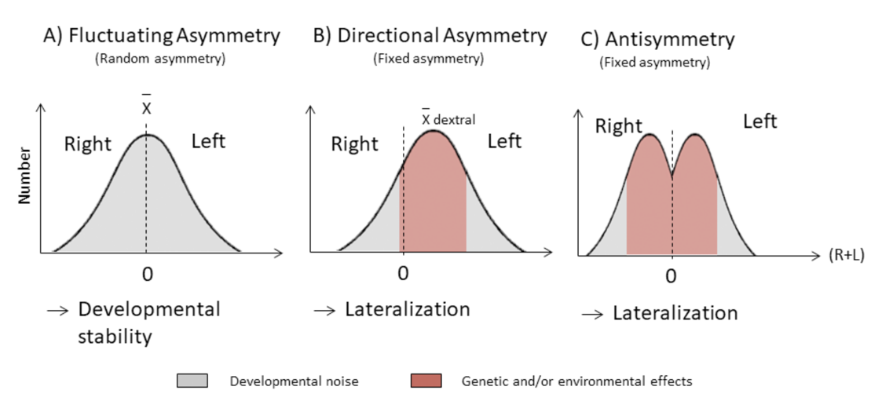
Fig. 3. Categories of asymmetry illustrated in three histograms (Mahé et al., 2021).
Horn development reflects the environmental conditions that the animal is subjected to. This is relevant for animals such as goats, whose horns continue to grow throughout their lifespan. To expand on the factors that affect horns, besides natural and sexual selection examined in the previous section, horn growth depends on changes in population density, climate, weather conditions and available resources. Scientists can observe how these factors influence horn development by analyzing the symmetry of horns within a population. We can quantify the variance from perfect symmetry by analyzing linear dimension variance and shape variance.
In general, fluctuating asymmetry is the standard deviation of the difference between the measurements of a trait on the left and right sides [di = li – ri]. FA is distributed around a mean of zero. In contrast, directional asymmetry is not distributed around a mean zero, but instead lies more on one of two sides. Finally, antisymmetry has a bimodal distribution about zero. Only DA and AS are found to be adaptive. However they typically reflect developmental issues (Parés Casanova & Kucherova, 2013).
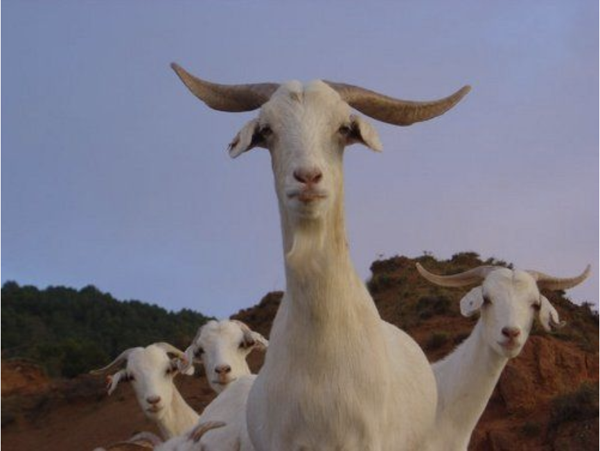
Fig. 4. Cabra Catalana goats. Medium sized animal with a skinny neck, long legs with short hair covering their bodies except for the long hair under their chin and along their upper thigh. Horns appear on both sexes; they are sharp and curved to the side and backwards, known as the Prisca type (Parés Casanova & Kucherova, 2013).
In a study performed by Parés-Casanova and Kucherova, the horn symmetry of Catalan Goats was observed. Their horns are illustrated in Figure 4. The research team studied each possible asymmetry using distribution plots. Fluctuating asymmetry is illustrated by a standard distribution curve centered at 0, and directional asymmetry is modeled the same but with a non-zero mean. Antisymmetry has two standard distributions, each with a non-zero mean of opposite signs. They used the Wilcoxan signed rank test to determine fluctuating asymmetry by comparing the difference in right and left sides with normal frequencies with a non-zero and a mean of zero. To determine antisymmetry they plotted cumulative frequencies against subtracted means of the differences. Skewness and kurtosis were also calculated. If the value of skewness is zero, it indicates that both sides balance out and are the same for an asymmetric or symmetric distribution. For example, an individual could have a fat and short tail but another could be long and skinny. Similarly, a large kurtosis value indicates a sharp peak favoring long and fat tails rather than short and skinny ones. The experimental design of the study involved collecting the total horn cord length and the basal circumference and analyzing horn asymmetry through distribution plots. Among the 27 female goats studied, the study puts forth the following data:
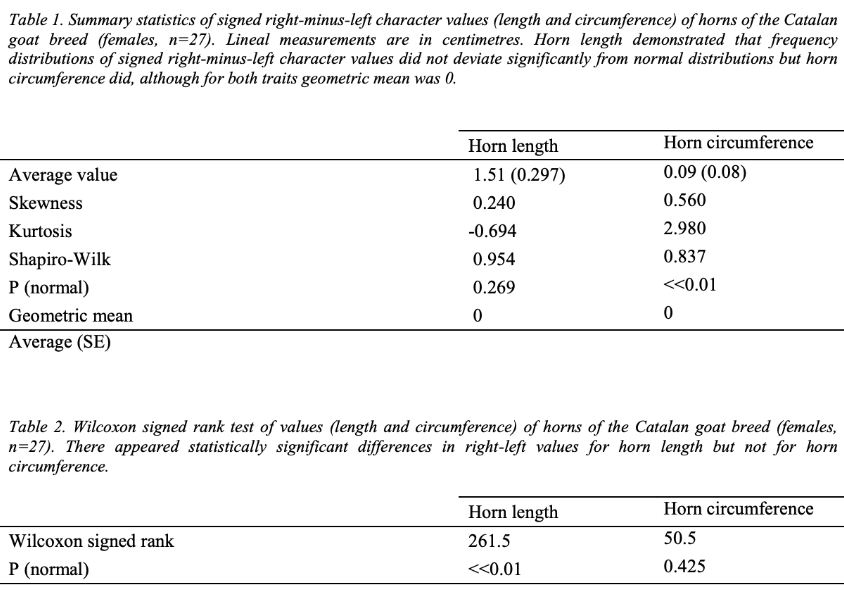
Fig. 5. Summary of the data collected in the study performed by Parés-Casanova et al. (Parés Casanova and Kucherova, 2013).
When analyzing fluctuating frequency using a mean of zero, the data suggests that horn length variations do not stray significantly from normal distributions as the p-value is greater than 0.01. This is not the case for horn circumferences, as the variations were statistically significant and varied largely from normal distributions. In contrast, the Wilcoxon test reveals a statistically significant difference between the right and left side lengths, however there is no difference in circumferences. Considering there is a low kurtosis value, it indicates that there is no one specific trait favored, suggesting a bimodal distribution. When plotting the cumulative frequency against the mean differences for both sides, Figure 7 reveals a graph with two straight-line plots confirming that horn length variations are antisymmetric (Parés Casanova & Kucherova, 2013).
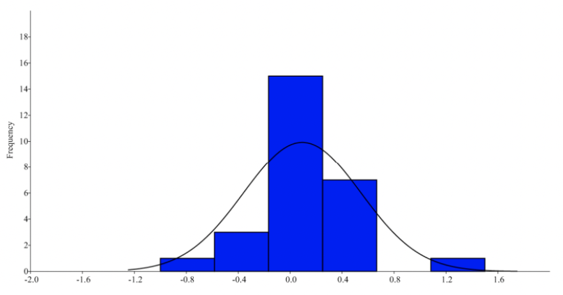
Fig. 6. Histogram of the circumference difference between the left and right side in Catalan goats (Parés Casanova & Kucherova, 2013).

Fig. 7. Cumulative frequency against the mean difference between the left-right lengths. Notice two straight-line plots and the change in modal distribution at the inflection point (Parés Casanova & Kucherova, 2013).
Given all the information known about horns and evolutionary selection, the interpretation of these results is tricky. Despite the data not supporting fluctuating non-adaptive asymmetry, intuitively it would make sense that a more symmetrical horn would be sexually selected for and result in a greater mating success while also increasing physical performance and survival. Moreover, skeletal asymmetry is associated with exogenous and endogenous factors such as genetics. That being said, antisymmetry may result from poor developmental conditions, heterozygosity, and inbreeding (Parés Casanova & Kucherova, 2013).
Nature’s favorite shapes
Mirror image pairs of helices
Helices are one of the most commonly occurring shapes in nature. They have elemental geometry and are enantiomorphic objects, meaning that a helix can have a mirror image pair which is identical in every area despite not being superimposable, like our right and left hand. A helix can be created by drawing a straight line on a piece of paper and then folding the sheet into a cylinder. Similar to a spiral, a helix is a coil which forms around a central axis in three-space. In biology, the helix is obtained when the spiral is a legalistic spiral defined by following equation (Galloway, 1989):
(r,d) = polar coordinates

Fig. 8. Example of helical structures in the living and nonliving world. a) spiraled seashells (Office National, 2022) b) double stranded DNA (Wheeler, 2007) c) spiral-horned antelope (Junek, 2022) d) spiral staircase in the Vatican Museum (NormanB, 2009).
By analyzing horned animals, it seems as though the helical shape of these appendages are closely related to the bilateral symmetry of their host. Neglecting asymmetrical distributions, mutations and other external factors sheep, goats and antelopes express enantiomeric pairs of horns, one right sided and the other left. Interestingly, in some species the right-handed helix is on their right side and in others it exists on their left side. This characteristic is labeled homonymous and heteronymous, respectively. The notable thing about this concept is that it reveals a relationship between the ectomeric nature of a pair of horns and the domestication of the animal. In general, wild animals are heteronymous and domesticated animals are homonymous. One researcher puts forth that spiraling horned animals were likely favored for domesticating since straight horned animals could be seen as more dangerous. Hence, animals with those less dangerous rapidly spiraled horns tend to actively live in homonymous (“similar”) pairs (Galloway, 1989).
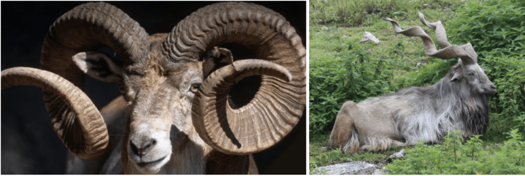
Fig. 9. Left image depicts a Bighorn Sheep (San Diego Zoo, 2022), and the right image depicts a Markhor (Schueman, 2022).
The natural logarithmic spiral
The Logarithmic spiral is a mathematical structure which characterizes many natural structures like horns, seashells, tails, and even galaxies. A logarithmic spiral has many fascinating properties, one of which is self-similarity. The spiral grows in a logarithmic fashion such that when “zooming” in or out it has the effect of endless continuation. In 2D polar coordinates the natural logarithmic spiral can be modeled as follows.
\begin{equation}
r=ae^{k\phi},\phi\;\epsilon\;R
\end{equation}
Where a and k are scaling constants describing the spiral’s growth properties in relation to the golden angle φabout the origin, and Euler’s number e.
Fig. 10. Ram horn (Left) clearly showing geometric similarity to a logarithmic spiral (Right) (Elsayed, M. 2021). The bottom image depicts the shell of Nautilus pompilius using a radiograph in the 20th century that illustrates the “equiangular” spiral of its shell, together with the arrangement of the internal septa (D’Arcy, 1945, p. 749).
Several mathematicians independently observed and quantified the logarithmic spiral, each describing it with unique properties. The logarithmic spiral was first observed as an “equiangular” spiral by Thompson D’Arcy, as illustrated by the iconic spiral of Nautilus pompilius shell (D’Arcy, 1945, p. 749). It was described as a spiral having a radius vector which intersects the curve with an equal angle at any point along the spiral. Later the same spiral was described by the definition of having segments which are scaled versions of each other, with equal scaling constants separating them. This property of self-similarity is vital in biology as it allows for continued structural growth and the addition of more segments of a structure without compromising the overall design. It allows horns to retain the strength and benefits of the spiral shape while continuously allowing for the horn to grow. The logarithmic spiral provides structural support to horns and a biological growth advantage because of self-similarity. The natural logarithmic spiral has some other interesting properties which can help us characterize the spiral and understand its place in nature (Harary, 2011).
In addition to being self-similar, interestingly, the spiral is also smooth, meaning the tangent is defined at every point. This includes the points very close to the origin. No matter how close one gets or how far one continues to zoom in, the spiral is infinitely smooth and self-similar. Additionally, stemming from self-similarity, the spiral is invariant to similarity transformations such as rotation, scaling, or translation. These transformations will yield the same spiral. These properties may be harder to reason with biology; however, it can be theorized that they provide a general and natural developmental advantage. This is generally discussed in biological architecture referencing the absence of straight lines in nature (Harary, 2011).
The Fibonacci sequence in nature
The fundamental building blocks of nature rely heavily on mathematics, in particular Fibonacci numbers. The Fibonacci sequence is found everywhere in nature, from pinecones, to pineapples, to single cells. Fibonacci numbers follow the sequence “0,1,1, 2, 3, 5, 8, 13, 21, 34, 55”. The sequence can be modeled by Fn = Fn-1 + Fn-2, and their ratio, also known as the golden ratio or golden number, is equal to 1.618034. Many biological patterns follow this sequence and maintain these ratio-forming spirals. (Kumari, 2016).
The Fibonacci sequence is heavily apparent in plants, however animals such as the Big Horn sheep exhibit such patterns in their appendages. To determine whether a structure is linked to the Fibonacci sequence a geometric construction can be performed. This begins with a golden rectangle which has dimensions which are Fibonacci numbers. The ratio of side lengths of these sides are the so-called “golden ratio”. Next, the rectangle can be divided continuously into smaller golden rectangle sections. Throughout these divisions, an arch is drawn through each new rectangle which will eventually result in a logarithmic spiral, as seen in Figure 10. The self-similarity of the logarithmic spiral is a beneficial biological property (Kumari, 2016).
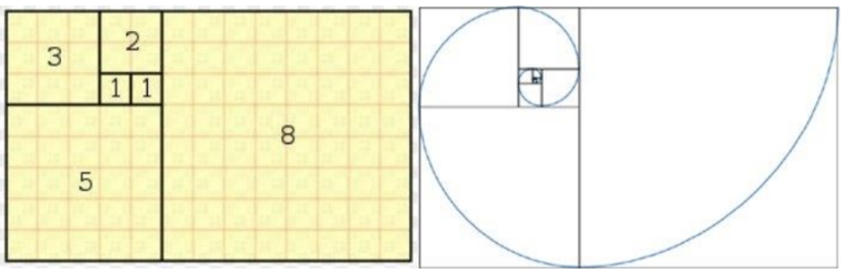
Fig. 11. Geometric construction of a Fibonacci or Golden spiral by creating golden rectangles and drawing arches within each division (Kumari, 2016).
The golden ratio represented by the greek letter Phi, φ, is closely related to many biological sequences and is in fact the limit of the ratio of Fibonacci numbers. The golden ratio, an irrational number, equals roughly φ = 1.618. It is quoted as being the most aesthetically pleasing ratio and is seen all over in nature. This ratio appears in many natural forms as a natural proportion, such as the length between nostrils (Abbas, 2017; Kumari, 2016).
The power cascade – an alternate horn growth model
With the discovery of the logarithmic spiral, Sir Christopher Wren theorized that shells follow this pattern, such that the pathway of the midline of the shell creates a logarithmic spiral (Wren, 1659). Since then, this approach has been used to represent shell growth. It is often expected that spiraled structures, including horns, follow this same growth pattern, since the principles behind modeling shell growth have been used in the past to model horn-like structures. However, upon further analysis, it seems that horn growth is better represented by a model called the power cascade (Evans et al., 2021).
The shape of pointed structures, such as horns, can be represented through the manner in which they grow by analyzing the rate of lateral expansion as the length increases (Fig. 12.). In one study, researchers modeled this phenomenon in teeth; however, it is mentioned that this model is easily applicable to other pointed structures, like claws, beaks, and of course, horns (Evans et al., 2021). Through 3D digitization of a tooth, researchers were able to measure this rate, by inspecting ten equally spaced cross-sections of the 3D tooth perpendicular to its midline (Fig. 12.a). The following equation represents the average radius of the cross sections (Evans et al., 2021).
\begin{equation}
Radius=\sqrt{\frac{A}{\pi}}
\end{equation}
A = Cross Sectional Area
Furthermore, by plotting the log of the radius (log10[Radius]) with respect to the log of the distance from the tip (log10[Distance]), the linear relationship modeled by Equation (9) arises. By manipulating Equation (9), it is clear that this relationship can be equivalently represented by Equation (10) (Evans et al., 2021).
\begin{equation}
\log_{10}(Radius)=Slope\times \log_{10}(Distance)+Intercept
\end{equation}
\begin{equation}
Radius=10^{Intercept}\times Distance^{Slope}
\end{equation}Moreover, it becomes apparent that this accord is a “Power Law” with a varying exponent (slope) and multiplier (10Intercept). When Slope = 1, the Distance and Radius measurements have a linear relationship, and when revolving this straight line around the x-axis, a classic cone is created (Fig. 12.a) (Evans et al., 2021). In other circumstances, when Slope = 0.5, the surface of revolution is a paraboloid (Fig. 12.c). As slope values fall under 0.5, the tip of the pointed structure is seen to become increasingly blunter. It is evident that the shape of the 3D modeled tooth is identical to the surface of revolution of a power function, otherwise known as a power cone (Evans et al., 2021). To describe the curved conical shape that cascades downwards according to the power function, this model is referred to as the power cascade. This model demonstrates a new class of shapes which vary in slope and intercept (Evans et al. t, 2021). The intercept acts as a scaling factor for the width of the pointed structure, in this case, teeth; a larger intercept leads to wider structures for the same length (Fig. 13.c) (Evans et al., 2021).
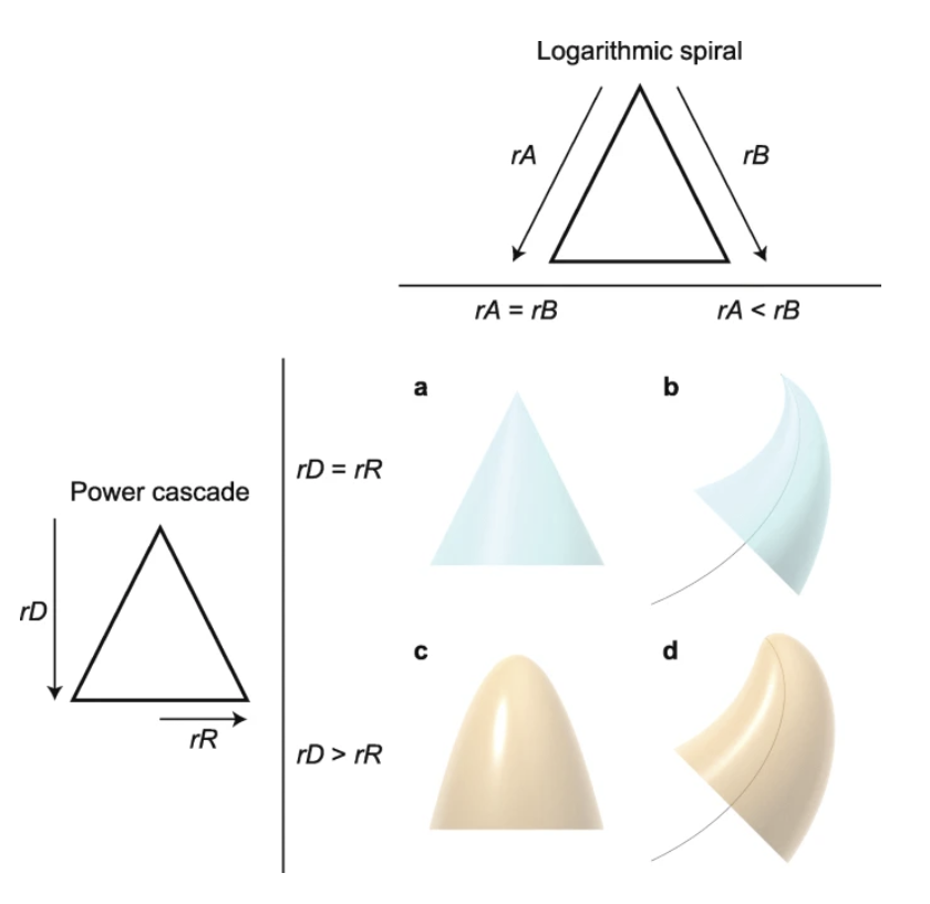
Fig. 12. Varying shapes of pointed structures, which demonstrate the effect of relative growth rates on shape. If growth rates (rA and rB) on both sides of a structure are equal, this results in a symmetrical structure, such as a classic cone a). If the growth rates are not equal, then the structure follows a logarithmic spiral (black curve) b). Equal power growth rates of the distance from the tip (rD), and radius (rR), result again in a symmetric cone a). When rR is less than rD, a power cone is produced c). In this case, rD=2rR, which creates a paraboloid. All these inequalities in growth rates can combine to form a power cone curving according to a logarithmic spiral, or a power curve d) (Evans et al., 2021).
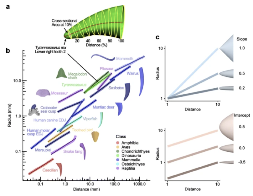
Fig. 13. Vertebrate teeth and other pointed structures like claws and horns grow according to the power cascade model, demonstrating linear change in log Radius with log Distance. (a) Example of measuring radius and distance for Tyrannosaurus rex tooth, which fits a linear model as seen in (b). (b) Teeth from other vertebrates also show a linear pattern on the log-log axis. (c) Power cones vary with respect to the slope (from conical to blunt) and intercept (from wide to narrow) (Evans et al., 2021).
As mentioned above, it was theorized that animal horn growth follows the shell or logarithmic spiral model. While this model is fairly successful, upon reevaluation, it is clear that the power cascade provides a more accurate depiction. If horns grew according to the shell model, and therefore were spiraled cones, then their slope would be equal to 1. However, by analyzing bony horn cores from vertebrates, it is revealed that they have a slope ranging from 0.4 to 0.8, which indicates that horn growth follows the power cascade model (Evans et al., 2021).
The majority of structures modeled by the power cascade tend to grow from tip to base, which is the case for animal horns (Evans et al., 2021). It is presumed that these shapes come about as the addition of material during growth increases the radius by a constant amount for a proportional increase in length. In terms of the reasoning behind this shape and model, it seems that many structures that can be modeled by the power cascade are used for penetrative purposes, such as animal horns, thorns, and claws. With this said, it is suggested that selection to maximize penetrative ability is the reason behind the similarities in shape as described by the power cascade (Evans et al., 2021). Nonetheless, there exist structures modeled by the power cascade that are not used for penetration, like rounded teeth or backward-curving horns. It also follows that structures that conform to the power cone can vary from sharp to blunt, so the underlying reason for structures modeled by the power cascade, is not necessarily caused by penetrative function (Evans et al., 2021). To this end, the most apparent explanation for the model fit is an underlying biophysical or developmental mechanism.
Applications of horn modelling
Using 3D finite element models for impact analysis
The skull and horns of bighorn sheep (Ovis canadensis) undergo large amounts of impact in intraspecific combat during ramming. These cranial appendages were evolutionarily designed to sustain massive dynamic forces while preventing brain damage and catastrophic failure. It is theorized that the combination of material composition and geometry are responsible for minimizing mechanical failure and factors that cause brain trauma (mainly, brain cavity translational acceleration) in these circumstances (Drake et al., 2016). In order to explore these hypotheses, dynamic 3D finite element models, approximation techniques which divide a complex space, into small segments, and whose behavior can be described by simple equations, were developed for the skull and horns to further understand the roles that horns and bone structures fulfill in energy absorption (Drake et al., 2016).
In particular, scientists took a mature male bighorn sheep’s skull and horns to develop an accurate geometry for the 3D model. Through X-ray computed tomography, a 3D imaging method which reveals information about the internal structure of materials, transverse slices of the skull and horn were obtained (Drake et al., 2016). Moreover, the numerous images of the inner layers of the horn were uploaded to 3D Slicer, a medical image analysis and visualization software, which ultimately defined the horn and bone regions and created a 3D surface model. The horns of Bighorn sheep are composed of a hollow curled structure, the keratin sheath, and a short, bony horn core. This software gave the model differing densities in the keratin vs. bone regions. The final 3D model and solution generation was designed by the explicit solver, ABAQUS 6.12, which is suited for dynamic contact simulations (Fig. 14.) (Drake et al., 2016). Furthermore, to further realize an accurate model, horn material and cortical bone regions were given material property values from literature values, and were assumed to be linearly elastic, isotropic, and homogeneous (Fig. 15.) (Drake et al., 2016).

Fig. 14. Finite element models. (a) Full Model: point mass and spine spring replicate and provide the mass and stiffness of a Bighorn sheep’s torso for a more accurate model. The arrows in this graphic are the initial velocity field applied which causes the horns to impact the plate. (b) Half Horn Model: same as the Full Model, but with exactly half of the horn length removed. (c) Model with Bone Removed: (left) same as the Full Model, but the trabecular bone can be seen within the horn; (right) same as Full Model, but with the horn core removed (Drake et al., 2016).

Fig. 15. Material properties utilized in the Horn model (Drake et al., 2016).
Model validation
To validate the element model, the dynamic, vibration response of the horn and skull structure was used. An experimental modal analysis (a study of dynamic properties) was performed on mature male horns using an impact hammer (Drake et al., 2016). In this experiment, three accelerometers were attached to the skull and horns; one on each horn tip, and one on the center of the skull. The horns and skull were stabilized with straps and springs to minimize the environmental vibrations. This apparatus was then impacted with an impulse hammer to generate natural frequencies (frequencies at which a system tends to oscillate naturally when disturbed) and mode shapes (deformations that the structure would show when vibrating at the natural frequencies) of the structures (Drake et al., 2016). The forces of the impacts were recorded, as well as the accelerations produced, and the natural frequencies were calculated. The most frequent natural frequencies that occurred were assumed to be dominant modes of the structure. Furthermore, two analyses on the 3D models were performed: an impact analysis and modal analysis (Drake et al., 2016).
For impact analysis (impact FE modal), horn-tip vibration was induced through impact in the model, with the same conditions as the model development discussed above. This impact was quantified as the oscillatory side-to-side displacements. This oscillatory displacement profile was broken down into two primary frequency components using Matlab. The horn-tip oscillation frequencies estimated through the model were compared to the experimental natural frequencies (Fig 16) (Drake et. alt, 2016).
Subsequently, a finite element modal analysis (FE modal) was carried out on a symmetric full-skull version of the model (Drake et. alt, 2016). The finite element model analysis predicted the natural frequencies and mode shape of the full skull, based solely on the geometry and material properties, which were then compared to the experimental natural frequencies similar to the impact model (Fig 16).
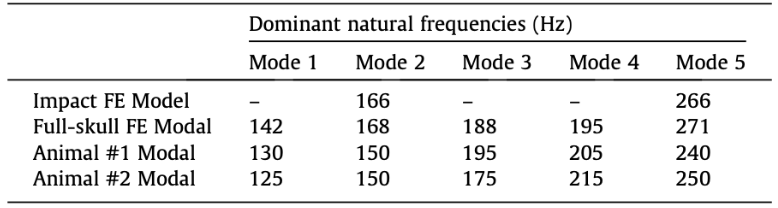
Fig. 16. Dominant natural frequencies results: (Row 1) horn tip oscillation frequencies induced by impact analysis in the Full Model dynamic simulation (Impact FE model). (Row 2) first 5 modes predicted by the finite element modal analysis on the Full Model. (Row 3-4) first 5 modes observed in real animal horns from experimental modal analysis (Drake et al., 2016).
As seen in the figure above, the experimental frequency modes matched the modes estimated by the mathematically produced models, using the finite element frequency analyses, which ensure structural and material validity of the finite element modal (Drake et al., 2016).
Other models
As seen in Figures 17b and c, two more models were produced to further investigate their function in the case of impact. The Half Horn (Fig. 17.b) model was made, where half of the horn length was removed, by eliminating the nodes and distal half of the horn (Drake et al., 2016). The other model (Fig. 17.c) consisted of a horn lacking the horn core trabecular bone. The same protocols, tests, and validation techniques were applied to these models.
Stress and strain analysis
During initial impact, the stress felt by Bighorn sheep horns is concentrated at the impact site. Since their horns are curled the impact site lies around the middle of the horn length (Fig.17a) (Drake et al., 2016). Around one millisecond after initial impact, the momentum causes the horn curl to load with compressive stress along the interior of the concave segment of the horn, and tensile stress along the exterior of the convex segment of the horn (Fig. 17.b). This stress propagates towards the tips of the horns (Fig. 17.c) and a torque is produced due to the geometry of the structure, which creates the side-to-side oscillations discussed above (Drake et al., 2016). In this scenario, the largest stress present in the bone is situated at the base of the horn core; high tensile stress is present in the front of the horn core base and high compressive stress in the back of the horn core base (Fig. 17.d & e).
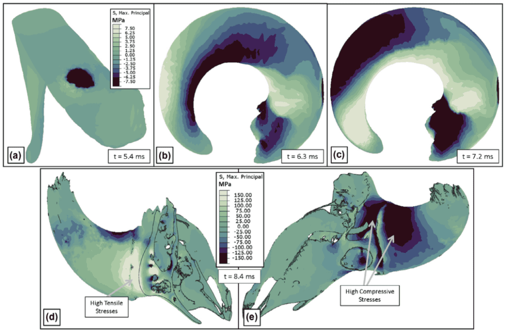
Fig. 17. Stress patterns: black indicates highest compressive stress and white indicates highest tensile stress. (a) Horn stress upon initial impact. (b) Horn spring-like behavior: compressive stresses on the inner concave surface and tensile stresses on the outer convex surface. (c) Tension and compression forces which induce side-to-side oscillations. (d) High tensile stresses at the base of the horn core on the impact side. e) High compressive stresses at the base of the horn core on the back side (Drake et al., 2016).
Since the validity of the 3D models is confirmed, the energy from the strain shown in Figure 18 and kinetic energy values were gathered for all the components making up the horn and bone material as a percentage of the total model energy (Figure 19) thanks to the Full 3D model (Drake et al., 2016). It was revealed that during impact, the bone stored 24% of the total energy, and the horn stored 8%, the rest of the energy exists in the point mass and spine spring mentioned above. The kinetic energy of the bone during impact dropped to almost zero due to its near zero velocity, while the KE in the horn during impact was 3.2%, due to the oscillations present in the horn, which create a larger amount of KE to dissipate the energy (Drake et al., 2016).

Fig. 18. Model horn and bone energy contributions (percentage of total model energy). Bone stores the largest amount of strain energy, while horn stores the largest amount of KE (Drake et al., 2016).
By further analysis of the Full 3D model to the modified models, this technology is also capable of quantifying the concussion and brain trauma variables, which consist of translational and rotational brain cavity accelerations (Drake et al., 2016).
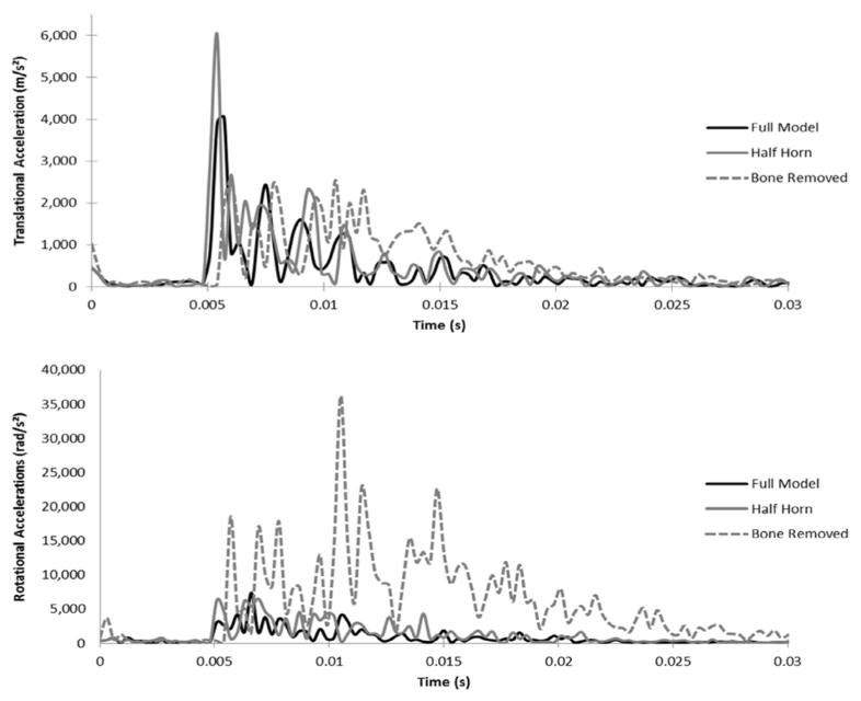
Fig. 19. Brain cavity movement and acceleration. (a) Translational Accelerations: The Half Horn model has a significantly higher acceleration peak during initial impact, while the Bone Removed model shows high peaks for a sustained duration. (b) Rotational Accelerations: Throughout the simulation, the rotational accelerations of the Bone Removed Model are much higher than the other models (Drake et al., 2016).
Ultimately, the Finite Element models and simulations, designed digitally through computational software and modeling an actual horn, are extremely effective at replicating material and geometric behavior in horns (Drake et al., 2016). This study uses carefully calculated modeling techniques to demonstrate how the shape and material of horns and horn core contribute to preventing brain injury during high impact head-on collision. This work allows for the understanding of material selection and design and a better comprehension of the evolutionary choices of many biological materials used in high impact scenarios (Drake et al., 2016). Through the assistance of these modeling techniques, it is possible to better design and manufacture energy dissipative structures, such as helmets, by observing and truly understanding the energy dissipative mechanisms and materials designed by nature – the ultimate engineer.
Computational modelling of yak horns
Generally, bovine horns are irregular curved cones with a larger proximal cross-sectional area and a smaller distal section. The mechanical properties of these keratinous structures are studied in detail. However, these investigations usually leave out information about how structural gradients affect these mechanisms. To this extent, a finite element method can be used to analyze stress and strain distributions of a horn model. This type of analysis can improve structural bionic design of horns (Liu et al., 2018). Problems which involve geometrical analysis cannot be achieved through traditional analytical methods such as partial differential equations. Alternative methods such as approximating partial differential equations using discretization methods must be used instead. The finite element method is used to compute these approximations by providing numerical model equations (Detailed Explanation of the Finite Element Method (FEM), 2016). Obtaining an accurate finite element solution depends on how accurately computer programs can approximate the stress or displacement influence functions of a finite element. These functions represent a structure’s response to an external load. Furthermore, finite element methods can provide a technique for substitute loadings, projection methods, and energy methods. The finite element method has a tremendous number of applications. In general, it involves studying structures with finite elements, which are constricted by their geometry and must be represented by shape functions, such as buildings (Hartmann & Katz, 2007).

Fig. 20. Yak horn Illustration in Bovine Animals (Bovine Horn Highlands, n.d.).
Applying this type of analysis to Yak horns involves measuring its radius, R. Next, the function of the curvature from the center of the horn is equal to 1/R , it is found as well as the continuous angle. The thickness of the horn is not uniform; however, its variation is insignificant compared to the overall size, so the thickness is used in the model. Next, the radius of the horn is a function of its angle r(θ). Finally, the mathematical model of the Yak horn is expressed as (Liu et al., 2018)
\begin{equation}
r(\theta)=a\left(\frac{\theta}{75}\right)+a_0
\end{equation}a0 = the geometry at the tip of the horn when the angle is 0
a = structural gradient (steepness) of the cone-like structure
A study performed by Yuxi Liu et al. analyzed a Yak horn with the following dimensions: R = 210 mm, h (thickness) = 5 mm, θ = 75°. In order to understand the relationship between structure and stress-strain, the study compares the stress and strain distributions of the horn when its structural gradient is different, as seen in Figure 21, with the actual parameters of a Yak horn (Liu et al., 2018).
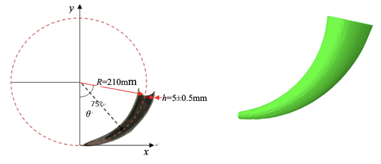
Fig. 21. a) Plane-coordinate system illustrating the symmetry plane of a Yak horn b) Analysis model of a Yak horn (Liu et al., 2018).
Yuxi Lieu et al. generated and analyzed four horn models with gradient distributions seen in Figure 22.
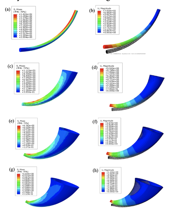
Fig. 22 Stress and strain distribution models of a Yak Horn (Liu et al., 2018).
Their findings suggest that a small steepness in a model generates a large stress concentration, decreasing the strength of the horned structure. Contrarily, when there is a large steepness, the stress and strain are concentrated at the tip of the model, which leads to material waste and does not convey a lightweight structural design. Based on the conical model of the Yak horn and the stress and strain effects in relation to its macroscopic gradient, Liu and their team concluded that there exists a gradient from the distal end to the proximal end in the axial direction of the horn. When an external load is applied to a horn of around 42 steepness, there is an increase in uniform stress and strain distribution, improving the strength of the structure. Finally, their data suggests a relationship between the toughness of horns and their structural gradients, indicating that a gradient steepness of 42 is the optimal bionic design (Liu et al., 2018).
Computational analysis of the 3D primordial folding of beetle horns
Glossary
- Primordial state of a horn: Initial un-grown stage at the structural level.
- Folding pattern: The physical process by which a protein chain is translated to its native three-dimensional structure.
- 3D Algorithmic meshing technique: The computational method for analyzing a 3D object relative to its various key structural and 3D features.
- Morphological changes: Changes in the appearance of the outer structure during development.
Horn morphologies and the Japanese rhinoceros beetle horn
Horns are biological adaptations with complex morphologies and patterns. To this degree, traditional experimentation is not a viable strategy to approach and analyze their folding patterns and their underlying causes due to the inability to artificially manipulate the folding patterns. However, the 3D morphology of a horn can be deciphered through understanding the relationship between folding and the 3D morphology itself. This form of analysis is performed using various 3D meshing algorithmic analyses that will be outlined in this section. The best way to apply these techniques is through top-down unfolding of a fully grown horn to its primordial state (Matsuda et al., 2021).
To that end, beetle horns, specifically the Japanese rhinoceros beetle called Trypoxylus dichotomus, as shown in Figure 23, were chosen as the case study species for their complex and compact folded horn. Moreover, beetle horns offered huge opportunities to probe the causes, mechanisms, and significance of phenotypic advances and diversification through their astonishingly diverse, evolutionarily unique, and ecologically significant sexual weapons their horns are (Kijimoto et al., 2013).

Fig. 23. Japanese Rhinceros Beetle, Trypoxylus dichotomus (David, 2022).
3D meshing algorithmic techniques
As mentioned, we need to link the folding pattern to the end 3D morphology to understand a horn’s shape. To that end, beetle horns’ overall folding patterns, to be deciphered, have to be analyzed on a computer for the primordial local folding at each different region and the contribution of how each individual region folding leads to the transformation into a fully grown horn must be related. Only by unfolding the primordium can the 3D shape of the end grown horn be understood.
On the other hand, to categorize each of those different regions and analyze their unfolding patterns, 3D meshing techniques are needed using computer algorithms to identify them. Firstly, we need to identify each region in the folded primordia that corresponds to the grown version of that region in the unfolded primordia, hence the “correspondence analysis” (red dotted line in Figure 24). In order to better investigate the furrow patterns, the surface can be smoothed and then the original mesh can be compared vs the smoothed mesh to identify the ridges and valleys characteristics of a furrow (blue dotted line in Fig. 24). Additionally, to understand the contribution of specific furrows to transformation, the unfolded state of the original mesh can be compared with the unfolded state of the smoothed surface, where the smoothed mesh had altered the furrows to be shallower allowing for this comparison (yellow line in Figure 24).
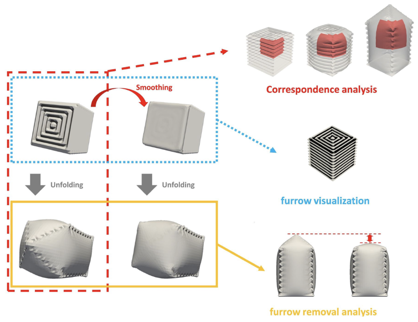
Fig. 24. 3D Meshing Methods for the Analysis of Furrows and Transformations, where the section discussed red-dotted line referring to the “Correspondence Analysis,” the blue-dotted line to the “furrow visualization,” and the yellow line to the “furrow removal analysis” (Matsuda et al., 2021).
Overview of morphological changes
To begin, it is important to categorize the major morphological changes between the primordial and grown states. In Figure 25a/b, the external shapes of the peeled larva i.e. the ungrown state and the pupal horn are compared for any differences; the figure reveals that the larva differ in the lateral width and dorsoventral length as well as the absence of the four-branched structure in the larval state. Finally, a closer look at the larva shows the complex furrow patterns in Figure 25d that would play a crucial role in the development of horn morphology (Matsuda et al., 2021).
Hence, the study by Matsuda et al. (2021) has attributed 3 of these different regions to 3 distinct structures to be simulated and studied individually: the cap, stalk, and the base. The main types of changes are in shape, length, and angle in the overall transformation.

Fig. 25. Overview of the differences between the Larval and Pupal Horn growth states which allow for the characterization of regions in the simulation (Matsuda et al., 2021).
Analysis of the base, stalk, and cap structures
Analyzing the base of the larva using furrow visualization technique and unfolding it as shown in Figure 26a reveals the discrepancy in the distribution of furrows on the ventral side in Fig.ure26b. Enlargement of this difference in the ratio of furrows shows the underlying mechanism attributed to the transformation of the base; in particular, the difference results in the orientation of the horn dorsally (Matsuda et al., 2021).

Fig. 26. Simulation analyses of the base structure of the larva’s horn growth site (Matsuda et al., 2021).
The middle part of the horn, the stalk, when in larval state, appears very small as in Figure 27a while being compact compared to the fully grown horn, but the folding features of the stalk in Figure 27d/e/f, such as the furrow patterns contributing to the elongation of the cylinder along the proximodistal axis, suggest passive formation as the longitudinal pressure creates the wavy folding in Figure 27d. The initial compact form of the stalk before growing into the lateral part of the horn is illustrated by the folding as in Figure 27g/d (Matsuda et al., 2021).

Fig. 27. Overview of the structure of the stalk in larval state and its furrow patterns that lead to its compact form before developing into a horn. In particular, the h and g are the corresponding analogous patterns of the furrows imprinted during primordial state of beetle horn versus its fully grown, vertically and horizontally (Matsuda et al., 2021).
Finally, for the top Cap structure of the horn, the contribution of the initial furrow patterns allows for the transformation of the primordial dome-like shape into the pupal four-branched defining shape of the horn. The furrow visualization and furrow removal analysis of both smoothed and original surfaces of the media tip as in Figure 28d/h/i/j/k influence the curvature of the branched structure into each of those branches as a result of the micro furrows seen in Figure 27I (Matsuda et al., 2021).
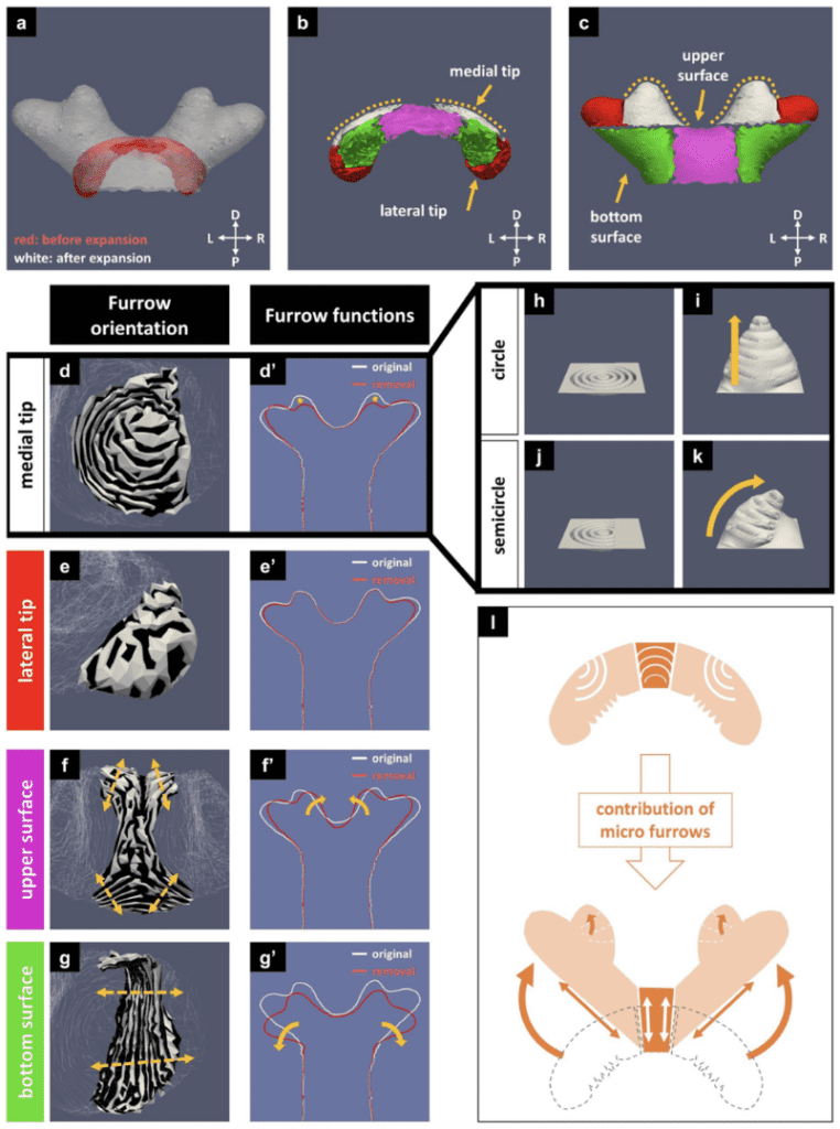
Fig. 28 Simulation of the Cap structure’s furrows contribution to the four-branched characteristic of the Beetle Horn, a) superimposed image of the cap before and after expansion, b,c) horn subdivided into regions before and after expansion d,e,f,g) furrow visualization of the cap h,i,j,k) concentric circle linear conical expansion compared to conical overhang concentric semicircle expansion (Matsuda et al., 2021).
Overview of the beetle horn growth as a result of the contribution of all 3 structures
Combining the impacts of each of those three regions reveals the distinct contribution of each to the overall morphology of the beetle horn, illustrated in Fig. 29. The base structure starts as a bellows-like fold and through its varying furrows is allowed to dorsally turn and develop the base of the horn. The next layer, the stalk, is initially in a zigzag compact folded state that elongates to form the cylindrical height of the horn. The final top layer, the cap, is actively defined by the inherent, present furrow patterns that shape the four-branched outreaching aspect of the beetle horn (Matsuda et al., 2021).

Fig. 29. Overview of the beetle horn growth due to the contribution of all three structures (Matsuda et al., 2021).
Therefore, this simulation of the development of the beetle horn through various analyzing techniques highlights the beautiful biologically engineered adaptation that from small primordial “patents” grows the durable and socially impactful structure that is the horn, without which an animal is crippled.
Conclusion
Most people believe that humans created math, that it did not exist before. That is debatable. Math is everywhere in the world around us and is evident in every aspect of the biological world. The naturally occurring arithmetic merely inspires humans, and it shows in the models, statistics, and shapes in everyday life. This paper demonstrates just one aspect of mathematical applications to biological structures, in this case the animal horn. Quantifying evolution reveals how the size of an animal’s ornamentation signifies their mating capital and acts as an honest advertisement for potential suitors. Computing the symmetrical pattern of animal horns reveals an antisymmetric relationship with a bimodal distribution curve. Furthermore, the patterns and curvatures of horned appendages are not random. As demonstrated throughout this paper, mathematical sequences and equations are riddled within these appendages. The first being nature’s numbers and spirals, the natural logarithmic spiral, the Fibonacci sequence and the Golden Ratio. The sequence of natural numbers and their ratios are expressed in several biological structures such as pine cones, pineapple skin, flowers, and DNA, to name a few. However, the Power Cascade may be a more accurate way of quantifying these structures by investigating the effect of relative growth rates on horn shape. Moreover, computational analysis can be used to describe the relationship between gradient steepness and horn strength. For instance, the Finite Element models and simulations of animal horns prove effective at replicating material and geometric behavior in horns. Finally, the primordial state in beetle horn is encoded by furrows distinctly at three regions that directly influence the development of the final 3D morphology of this well-engineered structure. This research makes it possible to better design dissipative technology by taking inspiration from years of evolutionary engineering in animal horns. In addition, the relationship between evolution, shape, structure and function is not random. It is approximated by a complex network of mathematical equations and theories that scientists are continuously trying to map out using computational analyses.
References
“Study Explains Evolution Phenomenon That Puzzled Darwin.” ScienceDaily, 30 Nov. 2016, www.sciencedaily.com/releases/2016/11/161130114158.htm. Accessed 16 Nov. 2022.
Clifton, Sara M., et al. “Handicap Principle Implies Emergence of Dimorphic Ornaments.” Proceedings of the Royal Society B: Biological Sciences, vol. 283, no. 1843, 30 Nov. 2016, p. 20161970, 10.1098/rspb.2016.1970.
Parés Casanova, Pere-Miquel, and Irina Kucherova. “Horn Antisymmetry in a Local Goat Population.” Repositori.udl.cat, 23 Dec. 2013, repositori.udl.cat/handle/10459.1/48084. Accessed 16 Nov. 2022.
Església, Carrer. “Pam a Pam | Cabra Catalana.” Pam a Pam, pamapam.org/ca/directori/cabra-catalana-vilanova-meia/. Accessed 16 Nov. 2022.
Mahé, Kélig, et al. “Directional Bilateral Asymmetry in Fish Otolith: A Potential Tool to Evaluate Stock Boundaries?” Symmetry, vol. 13, no. 6, 1 June 2021, p. 987, www.mdpi.com/2073-8994/13/6/987/htm, 10.3390/sym13060987. Accessed 17 Nov. 2022.
Galloway, J. W. (1989). Reflections on the ambivalent helix. Experientia, 45(9), 859–872. https://doi.org/10.1007/bf01954060
Drake, A., Haut Donahue, T. L., Stansloski, M., Fox, K., Wheatley, B. B., & Donahue, S. W. (2016). Horn and horn core trabecular bone of Bighorn Sheep Rams absorbs impact energy and reduces brain cavity accelerations during high impact ramming of the skull. Acta Biomaterialia, 44, 41–50. https://doi.org/10.1016/j.actbio.2016.08.019
“Tragelaphini.” Wikipedia, 16 Nov. 2022, en.wikipedia.org/wiki/Tragelaphini. Accessed 17 Nov. 2022.
“Helix-Turn-Helix.” Wikipedia, 11 Mar. 2022, en.wikipedia.org/wiki/Helix-turn-helix.
Norman, B. “English: Spectacular Spiral Staircase in the Vatican Museums in Rome (Italy) Designed by Giuseppe Momo in 1932.” Wikimedia Commons, 4 Aug. 2009, commons.wikimedia.org/wiki/File:Rome_-_Vatican_Museum_-_Spiral_Staircase_by_Giuseppe_Momo_-_0673_v2_cropped.jpg. Accessed 17 Nov. 2022.
“COLORIFIC FARMED SEA SHELLS ASSORTED 1KG | AASTAT Office National.” Www.officenational.com.au, www.officenational.com.au/shop/en/aastat/colorific-farmed-sea-shells-assorted-1kg-7074188i. Accessed 17 Nov. 2022.
Markhors: magnificent corkscrew horned goats living high in the Himalayas. (n.d.). One Earth. https://www.oneearth.org/species-of-the-week-markhor/
Goat and Sheep | San Diego Zoo Animals & Plants. (n.d.). Animals.sandiegozoo.org. https://animals.sandiegozoo.org/animals/goat-and-sheep
Liu, Y., Li, A., & Yan, G. (2018). Effects of structural gradient characteristics of yak horn on its mechanical properties. IOP Conference Series: Materials Science and Engineering, 439, 042002. https://doi.org/10.1088/1757-899x/439/4/042002
Hartmann, F., & Katz, C. (2007). Structural Analysis with Finite Elements. In Google Books. Springer Science & Business Media. https://books.google.ca/books?id=WSP9FsMWpAsC&printsec=frontcover&source=gbs_ge_summary_r&cad=0#v=onepage&q&f=false
Detailed Explanation of the Finite Element Method (FEM). (2016). Comsol.com. https://www.comsol.com/multiphysics/finite-element-method
Evans, A. R., Pollock, T. I., Cleuren, S. G., Parker, W. M., Richards, H. L., Garland, K. L., Fitzgerald, E. M., Wilson, T. E., Hocking, D. P., & Adams, J. W. (2021). A universal power law for modelling the growth and form of teeth, claws, horns, thorns, beaks, and shells. BMC Biology, 19(1). https://doi.org/10.1186/s12915-021-00990-w
Matsuda, K., Gotoh, H., Adachi, H., Inoue, Y., & Kondo, S. (2021). Computational analyses decipher the primordial folding coding the 3D structure of the beetle horn. Scientific reports, 11(1), 1-12. https://doi.org/10.1038/s41598-020-79757-2
Kijimoto, T., Pespeni, M., Beckers, O., & Moczek, A. P. (2013). Beetle horns and horned beetles: emerging models in developmental evolution and ecology. Wiley Interdisciplinary Reviews: Developmental Biology, 2(3), 405-418. https://doi.org/10.1002/wdev.81
David. “Japanese Rhinoceros Beetle Care.” David’s Beetles. David’s Beetles, May 13, 2022. https://davidsbeetles.com/blogs/news/trypoxylus-dichotomus-care.
Kumari, K. M. (2016). EXPRESSION OF FIBONACCI SEQUENCES IN PLANTS AND ANIMALS (p. 17). http://bomsr.com/4.S1.16/F5%2026-35.pdf
Guimarães, D. (n.d.). David Guimarães. Getty Images. Retrieved November 28, 2022, from https://www.gettyimages.ca/detail/photo/david-guimar%C3%A3es-royalty-free-image/999696758?adppopup=true
Harary, Gur, and Ayellet Tal. “The Natural 3d Spiral.” Computer Graphics Forum, vol. 30, no. 2, 2011, pp. 237–246., https://doi.org/10.1111/j.1467-8659.2011.01855.x.
D’Arcy W. T. (1945). On growth and form. University Press, Cambridge; Macmillan, New York. https://archive.org/details/ongrowthform00thom/page/748/mode/2up Bovine Horn Highland (n.d.). Retrieved December 13, 2022, from https://pxhere.com/en/photo/1612999