Abstract

The role of ungulates’ hooves, which are morphologically complex structures, is to support body weight and provide traction to aid in their adaptation to varied external conditions. This essay aims to investigate the relationship between the mathematical model and the morphology of the hoof. The golden ratio, an irrational constant discovered by ancient Greek mathematicians around 300 BCE, is used to determine the volume of the hoof and detect the center point of force based on the angle of the hoof. The magnificence of arithmetic is demonstrated by how contemporary math technology relates to ancient math. In the previous century, the bias cut became an innovation in women’s clothing, taking advantage of the diagonal pitch of textile fibers in a garment. The same structural principle is surprisingly also found in the hoof’s medium stratum, where the pitch of helices approximates 54 degrees. The helices of keratin in hooves inspire scientists on modern engineering design. The final section of the essay focuses on the rider and horse’s oscillatory motion while the horse is jumping. The graph of oscillation motion is generated using an inertial sensor, and it could be used to estimate the likelihood that an equine condition such as lameness is occurring.

Introduction

There are a few basic mathematical principles that govern life on Earth. The Fibonacci sequence is one such phenomenon. The Fibonacci sequence, also called the golden ratio or phi, begins like this: 0, 1, 1, 2, 3, 8, 21, …. Every term in the infinite sequence can be generated by taking the sum of the two previous terms. In nature, Fibonacci sequences can be seen in the number of flower petals in a flower, in shell spirals, or even in the spirals of galaxies, and many more. Perhaps a more unconventional application of the golden ratio is using it to calculate the volume of hooves, or even to represent the sum of the forces acting on the hoof. Hooves are not only governed by the Fibonacci sequence, but also by the special angle of 54⁰, which, like the golden ratio, can be found everywhere in nature. This angle represents the most stable arrangement of fibers in an orthogonal array which has been wrapped around a cylinder. This angle is found within the organization of keratin fibers in the hoof wall, but also in textiles, and fuel cylinders. Mathematical functions can be useful tools in understanding and modeling physical systems. For example, the sinusoidal function represents a continuous oscillatory movement. Sinusoidal functions can nearly perfectly model the interactions between a well-trained horse and rider and the movement of a horse with healthy hooves. In sum, the mathematical principles behind the Fibonacci sequence, the ‘magic’ angle, and functions can be used to understand the basics of many natural phenomena, including hooves.

The Golden Ratio

Part 1 of the Golden Ratio for Hooves: The Volume of Equines’ Hoof

Around 300 BCE, Greek mathematicians discovered and documented a phenomenon known as the golden ratio, which identified two values a and b such that a>b>0, and in which their ratio is equal to the ratio of their total over the bigger of the two amounts (Bejenaru & Babcinetchi, 2012). This occurrence can be observed in nature, art, architecture, and music (Iosa et al., 2018). In mathematics, the equation a/b=(a+b)/a=φ is used to express equality, with the Greek symbol phi (φ) representing the golden ratio. This constant satisfies the quadratic equation φ²=φ+1  and produces an infinitely irrational number that is roughly equal to 1.618 as a result (Marples & Williams, 2022). Geometrically, a series of squares with lengths corresponding to the Fibonacci sequence, in which each number is equal to the sum of the two numbers before it, can represent the golden ratio. This is illustrated in Figure 1 below (Benavoli et al., 2009), where the pattern appears aesthetically pleasing in the arrangement of the objects. Two alternative methods using geometric and mathematical models have been utilized to relate the golden ratio to the volume of an equine hoof (Gray et al., 2015). Modern mathematicians have developed the two approaches through integration and Archimedes’ work from 2000 years ago, The Method of Archimedes. The golden ratio is crucial in determining the volume of a hoof and may be calculated using either technique.

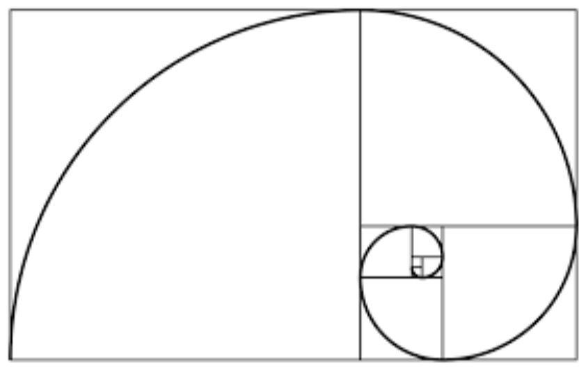
Fig. 1 The golden ratio diagram comprises a set of squares with lengths corresponding to the Fibonacci sequence (Markowsky, 2015).

Since the volume of the hoof is not a quantity that mathematical formulae can immediately compute, the first method in calculating the volume of the hoof breaks a cube with lengths of 2R into an ideal model of the equine hoof. As depicted in Figure 2, the hoof can be thought of as a section of a cube (Gray et al., 2015; Netz & Salto, 2001).

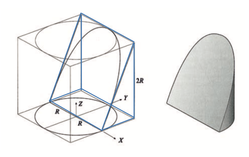
Fig. 2 The section of the equine’s hoof in a cube with a length of 2R where the blue lines represent the prism of the hoof from the cube in the left diagram. The extracted object illustrates the shape of the hoof in the right diagram (Gray et al., 2015).

It is necessary to clarify the coordinate system in order to compute the hoof volume. The surface of the sole is aligned on the diagonal cross-section across the xz-plane. The heel bulb is aligned on the x-axis and the center of the frog is located at the origin. The lateral side of the hoof is placed on the xy-plane; thus, the ideal model can be considered as the sole surface facing air. From -R to R, the side 2R is centered on the xy-plane. The z-plane varies between 0 and 2R. As a result, the hoof’s volume may be defined as:

V=\int_{-R}^R\int_0^{\sqrt{R^2-x^2}}\int_0^{2Y}dZdYdX

Eq. 1 The original equation of the volume of the hoof (Gray et al., 2015).

To be solvable, Equation 1 must be simplified. Thus, let x = X/R, y = Y/R, and z = Z/R, Equation 1 can be rewritten as

V=R^3\int_{-1}^1\int_0^{\sqrt{1-x^2}}\int_0^{2y}dzdydx

Eq. 2 The simplified equation of the volume of hoof.

Then by solving Equation 2,

\int_0^{2y}dz=2y

\int_0^{\sqrt{1-x^2}}2y\;dy=1-x^2

V=R^3\int_{-1}^11-x^2\;dx=\frac{4}{3}R^3

Eq. 3 The volume of the section of the hoof is found to be (4/3)R³.

V=2R\cdot2R\cdot2R=8R^3

Eq. 4 The volume of the cube with length of 2R.

Equation 4 provides a formula for calculating the volume of the cube containing the hoof segment, and the answer is 8R³. Consequently, V_hoof/V_cube is equal to 1/6.

In his 2000-year-old treatise The Method of Archimedes, Archimedes established the prior method (Waters & Addigis, 2015). The relationship between the volume of the hoof model and the volume of the cube with a length of 2R is established by the first technique.

In order to implement the second method, a single hoof model is used to integrate a triangle, a rectangle, or a segment of a circle on the x, y, or z planes, respectively, as shown in Figure 3.

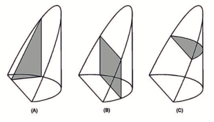
Fig. 3 The shaded areas represent the triangle in diagram (A), rectangle in diagram (B), and segment of circle in diagram (C), that is integrated in x, y, z plane respectively (Lynch, 2009).

The integration of diagrams A, B, and C in Figure 3 ought to provide the same answer using various methods:

V=\int_{-1}^1A\;triangle(x)\;dx=\int_0^1A\;rect(y)\;dy=\int_0^2A\;segment(z)\;dz

Eq. 5 The volume of equines’ hoof by integrating a triangle, rectangle, or segment of a circle, respectively (Lynch 2009). Note that A_triangle represents the area of a triangle, A_rect represents the area of rectangle (rect), and A_segment represents the area of a segment of a circle.

By expanding and solving the equation of area of triangle and rectangle, the following is obtained:

A_{triangle}(x)=1-x^2

Eq. 6 The simplified area of the triangle as written in Equation 5.

A_{rect}(y)=4y\sqrt{1-y^2}

Eq. 7 The simplified area of the rectangle as written in Equation 5.

As the triangular section in Equation 3 may be represented by Equation 6, then Equation 6 can be substituted into Equation 5 to determine the volume of the hoof, as shown in Equation 8:

V=\int_{-1}^1(1-x^2)dx

Eq. 8 The volume of the hoof found by substituting Equation 3 into Equation 6.

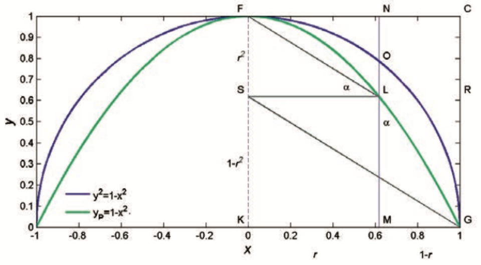
Fig. 4 The parabola of Archimedes Proposition 13, showing graphs y2+x2=1 for the purple line and y_p =  1-x² for the green line.

In Archimedes’ publication The Method of Archimedes in Proposition 13, he stated that the formula for a circle with a radius of one (1) could be derived from the equation y²+x² = 1 (Khrennikov 1990). The 2D equivalent of the parabola’s equation (in the xy-plane) is y_p= 1 – x², where y_p stands for a parabola’s equation. In Figure 4 of The Method of Archimedes, he developed the equation that MN²:MO² = MN:ML in the national form of ratio and proportion (Gray et al., 2015). The area of the y_p segment is equal to the volume of the hoof, according to Figure 4. Although the area of the parabolic segment is in two dimensions and the volume of the hoof is in three dimensions, this correlation may be explained by nondimensionalization, which implies that physical quantities like volume and area can be eliminated from one dimension by substituting the ratio (Alhama Manteca et al., 2012). As a result, the volume of the hoof can be reduced from 3D to 2D. As seen in Equations 6 and 7, the relationship between the areas of the triangle and the rectangle is known. The ratio is allowed to determine the volumes of the prism and hoof in Figure 1. Since A_rect/A_par = 3/2, V_prism/V_cube = 1/4, then V_hoof/V_cube = 1/6, and the first method is valid.

Once the golden ratio is used, the value of r in Figure 4 can fluctuate from 0 to R, which corresponds to Figure 1. The triangles GML and LSF in Figure 4 are similar; therefore, using the golden ratio equation, the result obtained is the inverse of the golden ratio, which is r = 1/ φ. Thus, MO = 1/√φ is obtained by changing the r value in The Method of Archimedes‘ equation.

Any hoof model that fulfilled the criteria from Figure 4 could be applied using the golden ratio, as long as the MO value was known, which is the measured length on the lateral side of the hoof. Therefore, the relationship between the ideal prism and real-world conditions can be examined using the hoof’s volume.

Part 2 of the Golden Ratio for Hooves: Kepler’s Triangle

A model of an ideal hoof is important for those concerned with equine locomotor biomechanics, or morphologies and is a key factor in the treatment of pathologies and diseases. Mario Livio, celebrated astrophysicist and author of The Golden Ratio: The Story of Phi, the World’s Most Astonishing Number (2002), states that “physical systems usually settle into states that minimize energy.” In nature, this leads to phenomena including logarithmic spirals and the golden ratio, so P.W. Balchin (2017) examined whether the phenomenon of the golden ratio – first discovered by Pythagoreans between 600 and 400 BC – held the key to optimal hoof dimensions.

Specifically, Balchin examined the “length of the dorsal wall, hair line to bearing border at the toe,” the “length of hair line to the last point of weight bearing at heel,” and the “length from the last point of weight bearing heel to toe at bearing border,” as seen in Figure 5 below. If the golden ratio presented itself in some form, Balchin stated that he would conclude that it was optimal as a product of evolution.

Fig. 5 The golden ratio in hooves (Balchin, 2017).

Balchin justifies the choice of these anatomical features, citing a study conducted by M.N Caldwells (2008) in which he relates their lengths to the golden ratio. Caldwells found that the Dorsal wall, the bearing border and a line segment joining the hairline on the Dorsal wall and the last point of bearing at the heel formed a perfect right angle. Additionally, Caldwells’ study found that in 16/22 feet, the values of the side lengths of the right-angle triangle formed a geometric sequence. This special case of side lengths that form a right triangle is known as Kepler’s triangle. See Figure 6 below for an illustration.

Fig. 6 Illustration of a Kepler triangle (Accessed November 15, 2022 from Wikipedia).

The ratio of the three side lengths of Kepler’s triangle is 1 :√φ : φ, where is φ the golden ratio, approximately equivalent to 1.618. It follows that the ratio of the area of the squares created by the progression is 1 :φ : φ². In his own study, Balchin used software to position Kepler’s triangles onto the cross-section of the middle of hooves. The bases for the fit of the triangles were the center points of the outside triangle, and the results can be seen in Figure 7 below.

Fig. 7 Kepler’s triangles fitted onto a cross-sectional image of a hoof (Adapted from Balchin, 2017).

Balchin noticed that the triangles had interesting properties. The center of one triangle was created where the “Deep Digital Flexor Tendon inserts into the semilunar crest on the solar surface of the Distal Phalanx” and that the center of another triangle represented the “point of force” of the hoof (Balchin, 2017). Unfortunately, Balchin did not label their diagram. 

Since they were fitting models onto images, there was a degree of error in Balchin’s fits. Their randomized study included 50 pairs of feet in a variety of breeds, ages, sizes, and causes of death. 59% of the hooves had a hairline angle of 90° as seen in Figure 7. A further 7% were within 1° of 90° and the range of angles was 82.4° – 100.4°. The mean hairline angle of all 100 feet was 90.644°, the median was 90.150° and the mode was 90°. The standard deviation was 2.993° and the variance was 8.959° (Balchin, 2017). The histogram in Figure 8 below illustrates the distribution of angles at the hairline of all the sample feet.

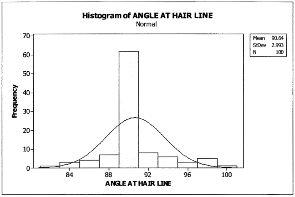
Fig. 8 Histogram of the angles at hairline: the angle formed by the dorsal wall and a line segment joining the hairline on the Dorsal wall and the last point of bearing at the heel. See Figure 5 and the paragraph below Figure 5 (Balchin, 2017).

Balchin proposed that the golden ratio and the 90° value at the hairline angle may be important when considering the forces that the hoof experiences. In Figure 9 below, Balchin states that the squares of the two shorter side lengths of the triangle represent a specific magnitude of load-bearing forces. Due to Pythagoras’ theorem, this magnitude is equal to the normal reaction force experienced by the bottom of the hoof, which is represented by the square of the side length, which is parallel to the ground. If the right angle does not exist, it would displace the center of the smaller triangles in Figure 7 which would mean that the forces are not transferred through the deep digital flexor tendon and the point of force (X and Y, respectively, in Figure 9 below). This could possibly increase the risk of pathological and morphological changes to the hoof and the structures surrounding it. As such, Balchin recommended that shoeing protocol in equine should be implemented by caretakers in such a way that, referring to Figure 7, the outside and inside triangles remain intersecting the digital flexor tendon and point of force.

Fig. 9 Diagram of forces experienced by the hoof through the perspective of Pythagoras’ theorem (Balchin, 2017).

Balchin concludes his study by stating that none of the hooves were trimmed specifically to fit the golden ratio. They stated that the golden ratio may have a role to play in search of the optimum hoof proportions, however, they suggest that it should be used as a guideline that someone who is trimming hooves can use in conjunction with other methods that have already been established.

Hooves, Orthogonal Arrays, and Helices

A fabric made of orthogonal fibers can be strategically oriented in a structure such as to maximize its desired properties. In fact, orthogonal arrays can be modeled to grasp mathematical concepts through clothing. The properties of such a material will be presented first, then a discussion about the strong keratin fibers that build the tubules of the hoof horn will be conducted. Finally, the importance of this structure will be discovered through the many appearances of orthogonal arrays and helices in nature.

In post-war society in the early 20^th century, clothing was made from textiles which were not stretchy – like cotton, linen, and silk. Further, fabrics were oriented such that the fibers extended circumferentially around, and vertically up and down the body of the wearer. Laces and ties, such as in corsets, were used to tighten the fabric around the body and to achieve a close-fitting garment, although this would introduce unwanted creasing (Gordon, 1978). Then, in Paris in 1922, designer Madeleine Vionnet invented a revolutionary method in the world of fashion – the bias cut. This is when the fabric is aligned such that the transverse and longitudinal threads are oriented at ± 45⁰ with respect to the horizontal and vertical (Fig. 10). Such an alignment gives the clothing the same properties in both the horizontal and vertical directions, and consequently increases the stretchiness in these directions (Gordon, 1978). This invention improved the drape of fabrics over women’s bodies, which have a non-uniform, non-cylindrical, and non-rectangular shape.

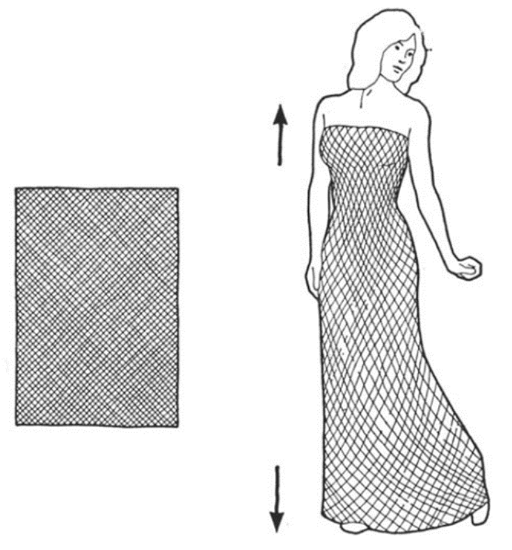
Fig. 10 If the cloth is pulled ‘on the bias’ or at ± 45⁰ to the warp and weft, the ‘material’ is extensible, and the Poisson’s ratio – and hence the lateral contraction – is large. This is the basis of the ‘bias cut’ in dressmaking (Gordon, 1978).

A few definitions are required to understand the properties of these helical materials. First, when a ‘rigid’ 2D lattice is constructed, a high stiffness in shear means that shear – causing either tension or compression at ± 45⁰ – will not cause the material to collapse (Fig. 11). Such materials are called isotropic, meaning they display the same properties in all directions. For example, glass is isotropic, and so is metal. On the other hand, anisotropic materials display different properties depending on the direction, and will collapse under high shear. For example, cloth is highly anisotropic. Second, Poisson’s ratio, nu (ν), is defined by the transversal elongation (x-direction) divided by the amount of axial compression (y-direction), and typically ranges from 0.0 to 0.5. For example, materials which collapse under compression have a Poisson ratio closer to 0. Young’s modulus (E) is a measure of elasticity, equal to the ratio between the stress acting on a substance and the strain produced. 

Young’s modulus and the shear stress of a material come into play when the orthogonal array is transposed onto a three-dimensional surface. Gordon (1978) explains that “for an initially flat membrane to conform easily to a surface with pronounced two-dimensional curvature, it is necessary to have both a low Young’s modulus and a low shear stress.” This means that flexible materials (low Young’s modulus) can easily be deformed by pulling or pushing along the axis, which runs at ± 45⁰ to the fibers of the material.

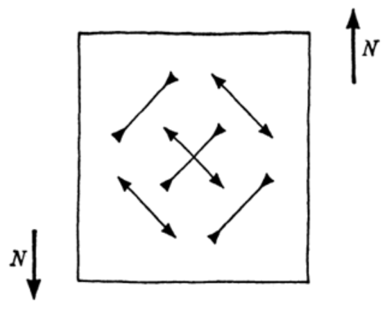
Fig. 11 Shear will produce tension and compression stresses in directions at ± 45⁰ to the plane of shearing (Gordon, 1978).

There is a geometric transformation that must be considered when augmenting a structure from 2D to 3D. When an orthogonal array is splayed in 2D, such as in a flat woven fabric, the angle formed between the fibers and the horizontal is ± 45⁰. When such a structure is rolled around a cylinder, the mathematically conventional optimal angle that prevents delamination and buckling due to an applied load is not 45⁰, but is 54⁰. This change in angle accounts for the curvature of the surface. A model can be visualized in Figure 12. The vertical length required for the helix to wrap once around the cylinder is the ratio between the circumference of the cylinder and the tangent of the angle of the coil with respect to the vertical, as seen in Equation 9 (Ferreira, 2006). Note that θ in this equation is the difference between 90⁰ and the angle with respect to the horizontal (the complementary angle).

L=\frac{2\pi r}{\tan\tan(\theta)}

Eq. 9

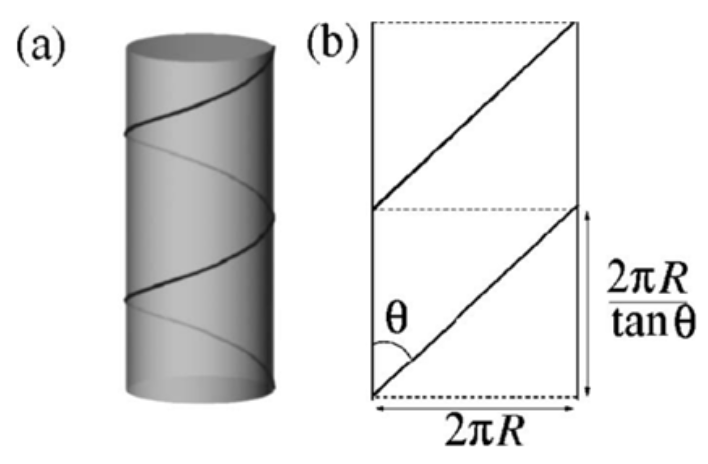
Fig. 12 Schematic diagram of the geometry involved in helical wrapping. (a) A single strand is assumed to wind around a cylinder of radius R at an angle θ. (b) In the two-dimensional depiction, the unwrapped tube is represented by a stripe of width 2πR and the coiling angle θ defines a unit cell of length 2πR/tanθ (Ferreira, 2006).

Using this equation, the ratio between the length of the cylinder when θ is 45⁰ and when θ is 36⁰ (the complement; 90⁰ – 54⁰) is 0.7265. This means that the length of the cylinder must be greater when the helix becomes more vertical. Another visualization is displayed in the following geometric models. Here, the constant alpha (α) is the inner angle of the parallelogram, and the variable beta (β) is the ½ angle of the dihedral formed by the outer surfaces of the parallelograms (Fig. 13).

Fig. 13 A folding motion of  the Miura-ori vertex (Tachi, 2010).

In Figure 14, the structure is mostly geometrically symmetrical, and is thus the soundest in the third configuration when α = β = 45⁰ (Tachi, 2010). In Figure 15, the structure is most geometrically symmetrical when α = 54⁰ and β = 67.5°. The important difference between these angles is that the structure is more elongated when α = 54⁰. Therefore, in materials where the function of the structure is to travel transverse distance, such as tubules, this larger angle of 54⁰ is optimal.

Fig. 14 The cylinder of α=45° at β = 89°, 67.5°, 45°, 22.5°, 1° (from left to right) (Tachi, 2010).

Fig. 15 The cylinder of α=54° at β = 89°, 67.5°, 45°, 22.5°, 1° (from left to right) (Tachi, 2010).

The mathematics between this change in angle is quite simple. Since the fibers wrapping around the cylinder are assumed to be inextensible, the length of fiber required to turn once around the cylinder is constant. Therefore, the volume of the cylinder is only a function of the length of the fibers, and consequently of their pitch angle (Horgan & Murphy, 2018). The volume enclosed by the fibers occurs when the derivative of the volume with respect to the angle is zero, or equivalently can be written as Equation 10:

2\cdot(\theta)-(\theta)=0

Eq. 10

Which yields Equation 11:

\theta=\arctan\left(\sqrt{2}\right)=\arcsin\left(\frac{\sqrt{2}}{3}\right)=\arccos\left(\frac{1}{\sqrt{3}}\right)\approx54.74\degree

Eq. 11

This purely mathematically- and geometrically derived angle appears frequently in structural elements of biological systems and is found in both “circular cylindrical tubes or cylinders reinforced by helically wound fibers” and “flat thin sheets reinforced by fibers in the plane” (Horgan & Murphy, 2018). Incredibly, hooves display this “magic” angle in both situations. 

In hooves, the middle layer of the horn wall, the thickest layer, is composed of intertubular material and horn tubules. Inside the horn tubules, crystalline fibrous α–keratin form helices (Figure 16). These helices increase the strength of the structure. While the horn tubules are essentially cylinders running straight and parallel to each other, the intertubular material forms laminated structures which cross the tubular axis at angles between 30° and 60° (Figure 17). These angles optimize the strength of the hoof wall – preventing buckling of the hoof when the weight of the animal is applied – and preventing cracks from propagating linearly (Wang et al., 2020). Therefore, the keratin helices inside the tubules and the angles formed between the sheets of laminated intertubular material are an ingenious occurrence of the principle of the “bias cut” in nature.

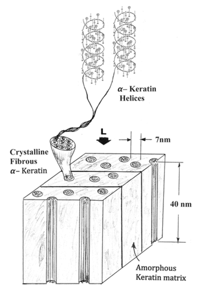
Fig. 16 Schematic views showing general structure hierarchy of horns. Hoof structure is similar. Elliptical tubules of α-keratin embedded in protein-based (keratin) amorphous laminar matrix. The arrow marked L illustrates applied compressive load acting on horns or hooves (Murr, 2015).

Fig. 17 Schematic of a hypothetical model to explicate the structure of the bovine hoof wall. (Wang et al, 2020).

Similarly, collagen fibers are a tough protein-based structure that stiffen tissues at high strains and contribute to their toughness (Gordon, 1798). In intestinal parasites, helical collagen fiber bundles wrap around the body of this hydraulic worm, forming the cuticle (Gilpin et al., 2015). These helices are wound around their bodies at approximately 54° and allow the parasites to have both a protective exoskeleton (which is subject to both internal and external pressures) and to wiggle, bend, and elongate inside the food source. This extension or compression comes from a variation in the angle between the intersecting fibers of the lattice (Clark & Cowey, 1958). In terms of engineering applications, knowledge about the properties of the lattice structure can be applied to cylindrical objects. For example, starting in about 1950, cylindrical cases for rocket propellant were wound from a double helix of glass fibers, and bonded together with a resin adhesive. As a consequence, the cylinders did not expand much circumferentially, but rather elongated, which was less damaging to the propellant (Gordon, 1978). By mimicking biological structures, the desired properties of cylindrical or helically wound objects can be optimized, while reducing the unwanted effects. Clearly, the fundamental properties of helically wound or lattice-based structures are the same between post-war fashion, hooves, the intestinal parasite, engineering applications and many more occurrences.

A mathematical model for the interaction of a rider and horse during a jump

A mathematical model is a description of a system using the language of mathematics as the primary way to explain the response and interaction of that system. On the other hand, a system is defined as a group of interacting elements that produce the desired outcome.

An example of how mathematical models can be used around the topic of horses and hooves is understanding the horse-human interaction that occurs during a jump and predicting the positions of the horse and the rider. During a horse-riding jump, the vertical position of the rider and the horse highly depends on the experience and skills of the rider and horse (Tsuruo et al. 2020). Also, the rider is subject to oscillatory properties before, during, and after the jump. Such oscillatory movement is characterized by amplitude, frequency, and phase. However, the horse also experiences an oscillation with respect to the ground, which can be expressed as a different oscillatory function. Since there are two objects in the system, the rider and the horse, a two-part model can better describe the desired outcome. The simplest model that can be used in this situation is a spring-mass-damper model. In this case, there are two spring-mass-damper models connected, one for the horse and another for the rider, both interacting with oscillatory functions representing the movement on the jump (Tsuruo et al. 2020). The use of the spring-damper model allows for including different variables that can be easily changed, meaning that the model can be easily applied to different horses or riders only by changing the parameters. Furthermore, by using two models, a contact factor can be included in the calculation to account for the interaction between the legs of the rider and the horse. 

The model can be graphically seen in Figure 18:

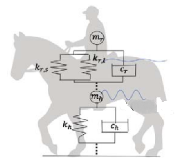
Fig. 18 Model for rider-horse interaction (Tsuruo et al., 2020).

The mathematical description of the models are the followings:

1. Model representing the rider’s motion:

The rider’s model contains two different springs and can be represented by Equation 12 (Tsuruo et al. 2021):

m_rz_r''=-n_{r,c}c_r\left(z_r''-z_h''\right)-n_{r,s}k_{r,s}e_{r,s}-n_{r,l}k_{r,l}e_{r,l}-m_rg

  Eq.12  

Where:

Figure 19 shows the model for the rider with a sinusoidal function representing the movement.

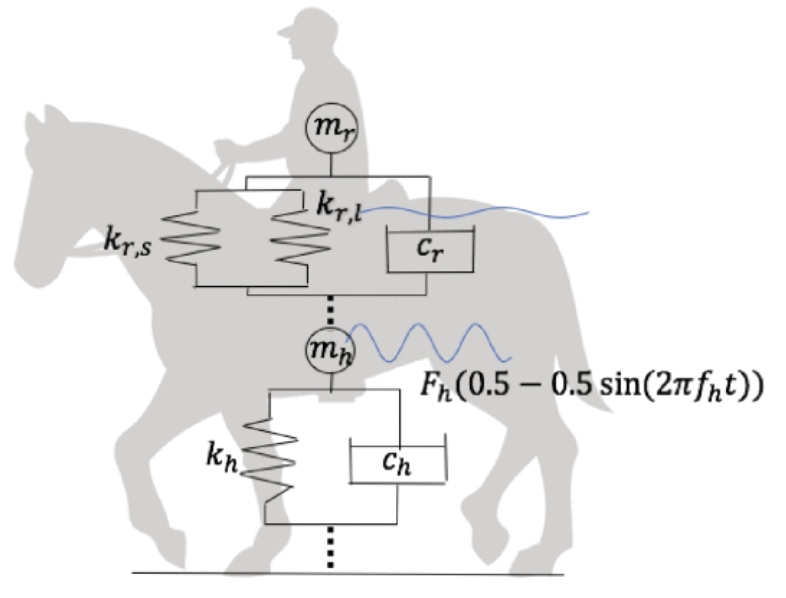
Fig. 19 Model for the position of the rider (Tsuruo et al. 2020).

As it can be observed, there are many variables on the model, which allows to have more accurate results and use the model for different riders and horses. However, many calculations must be done before having a functional model since all constants except the position of the rider must be determined.  

Using Python to solve the above equations and given parameters related to the experiment, Tsuruo and his colleagues were able to successfully use this model to estimate the position of the rider for two different data sets, as shown in Figure 20:

Fig. 20 Prediction of the position of the rider by the developed model comprising two data sets (Tsuruo et al. 2020).

2. Model representing the horse’s motion:

The horse’s position is modeled by a simple spring through Equation 13 (Tsuruo et al. 2021):

m_hz_h''=-n_hc_hz_h'-n_{r,s}c_r\left(z_r'-z_h'\right)-n_hk_he_h+n_{r,s}k_{r,s}e_{r,s}+n_{r,l}k_{r,l}e_{r,l}-m_hg+n_hF_h

Eq.13

Where:

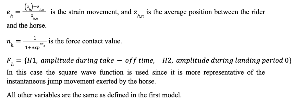
Figure 21 shows the model with the appropriate function as the input of the system.

Fig. 21 Model for the position of the horse (Tsuruo et al. 2021)

Again, using Python to solve the above equations and given parameters related to the experiment, Tsuruo and his colleagues were able to successfully use this model to estimate the position of the horse for two different data sets, as shown in Figure 22. The figure also shows the data obtained from the first model. It can be observed that using both models, a better understanding of the interactions between the horse and riders can be found. The models are a good approximation for the observed data, meaning they could be used to estimate values for different purposes.

Fig. 22 Prediction of position of the rider and horse by the developed model with two data sets (Tsuruo et al., 2021).

Inertial Sensors

As explained in the previous publication made by the authors “From Fetus to Fossil: A Microscopic Analysis of the Chemistry of the Hoof Throughout the Stages of Life”, lameness is a disease that affects the way an animal walks. Different studies show that the position of the head and pelvis in relation to the horse’s gait are two indicators for the early development of the disease (Schoeggl, 2017). A quick and non-invasive way to check these indicators is by using inertial sensors on the head and pelvis of the horse and observe the changes in the movement on those areas. Figure 23 shows the position of those sensors.

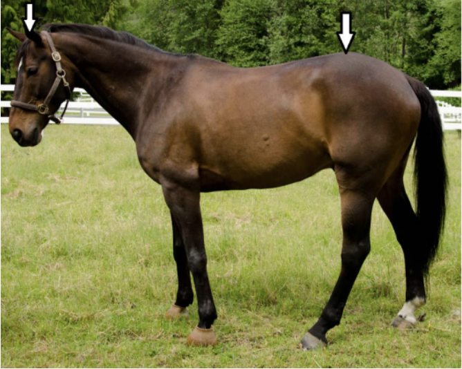
Fig. 23 Position of inertial sensors (Schoeggl, 2017).

The sensors record data at a high rate of about 200 frames per second and the points are graphed as vertical displacement with respect to time. Figure 24 shows the data given by the sensors of a healthy horse (Schoeggl, 2017):

Fig. 24 Data provided by the sensors (Schoeggl, 2017).

In order to determine if the horse is diseased, the sensors record the data and then compare it to the graph shown in Figure 24. The error of the obtained data can be calculated with the following formula (Equation 14) (Schoeggl, 2017):

Error=\frac{\partial x}{\partial y}

Eq. 14

where x(t) is the function representing the healthy data, and y(t) the function of analysis.

With the given graphs and the error, the veterinarian performing the diagnosis can determine if the horse is demonstrating early signs of disease or not. The threshold of error that shows the presence of lameness depends on multiple factors and only a professional can determine the horse’s condition (Schoeggl, 2017). This is a simple example to show how simple data recording, as the movement of the head and pelvis, can be helpful to determine the presence of a disease that can cause huge damage to animals.

Conclusion

In conclusion, mathematical principles that govern the universe can be applied to gain a deeper understanding of the physical and chemical properties of the hooves. In this paper, it has been proved that the golden ratio discovered by Greek mathematicians can be used to successfully estimate the volume of the hoof. An interesting relationship between the golden ratio and Pythagorean theorem on the hooves has also been found. Later, a comparison between the orthogonal arrays and helices on clothes and hooves helped to better understand the flexibility of the materials and the shear forces they can support. Mathematical models, based on physical concepts such as spring and damped oscillatory movements, gave an explanation as to how the rider and the horse interact during a jump. The model was also able to successfully predict the vertical position of both the horse and rider throughout the duration of the jump. Inertial sensors also showed how mathematical models could be applied to detect diseases such a lameness in their early stages. Mathematics is a useful tool that allows scientists to gain a deeper understanding of the biological world, and can be used to create new objects and improve quality of life.

References

Alhama Manteca, I., Soto Meca, A., & Alhama, F. (2012). Mathematical characterization of scenarios of fluid flow and solute transport in porous media by discriminated nondimensionalization. International Journal of Engineering Science, 50(1), 1–9. https://doi.org/10.1016/j.ijengsci.2011.07.004

Balchin, P. (2017). The Golden Ratio In Relation to Hoof Capsular Geometry In Front Feet §y. https://www.wcf.org.uk/fwcfthesis?tid=12cac84659fb5f982db319254d283d73e4e8c4053 7d10dba334229fb45fbed8c

Bejenaru, L., Babcinetchi, V., & 11th International Scientific Conference on Engineering for Rural Development Jelgava, LVA 2012 05 24 – 2012 05 25. (2012). “rediscovery” of the golden section (ratio) in byzantine art. Engineering for Rural Development, 11, 609–613.

Benavoli, A., Chisci, L., & Farina, A. (2009). Fibonacci sequence, golden section, Kalman filter and optimal control. Signal Processing, 89(8), 1483–1488. https://doi.org/10.1016/j.sigpro.2009.02.003

Clark, R. B., & Cowey, J. B. (1958). Factors controlling the change of shape of certain nemertean and turbellarian worms. J Exp Biol, p 731 – 751. https://doi.org/10.1242/jeb.35.4.731

Ferreira, M. S., & Wall, A. (2006). Electronic contribution to the energetics of helically wrapped nanotubes. Phys. Rev. B 74(233401). https://doi.org/10.1103/PhysRevB.74.233401

Gilpin, W., Uppaluri, S., Brangwynne, C. P. (2015). Worms under Pressure: Bulk Mechanical Properties of C. elegans Are Independent of the Cuticle. Biophysical Journal, 108(8), 1887-1898. https://doi.org/10.1016/j.bpj.2015.03.020.

Gordon, J. E. (1978). Structures or Why things don’t fall down. Penguin Books. https://doi.org/ 10.1007/978-1-4615-9074-3.

Gray, S. B., Ye, D. D., Gordillo, G., Landsberger, S., & Waldman, C. (2015). The method of archimedes: propositions 13 and 14. Notices of the American Mathematical Society, 62(9), 1036–1040. https://doi.org/10.1090/noti1279

Horgan, C. O., Murphy, J. G. (2018). Magic angles for fibrous incompressible elastic materials. Proc. R. Soc. 474. http://dx.doi.org/10.1098/rspa.2017.0728.

Khrennikov, A. Y. (1990). Mathematical methods of non-Archimedean physics. Russian Mathematical Surveys, 45(4), 87–125. https://doi.org/10.1070/rm1990v045n04abeh002378

Iosa, M., Morone, G., & Paolucci, S. (2018). Phi in physiology, psychology and biomechanics: The golden ratio between myth and science. Biosystems, 165, 31–39. https://doi.org/10.1016/j.biosystems.2018.01.001

Markowsky, G. (1992). Misconceptions about the golden ratio. The college mathematics journal, 23(1), 2-19.

Marples, C. R., & Williams, P. M. (2022). The Golden Ratio in Nature: A Tour across Length Scales. Symmetry, 14(10), 2059. https://doi.org/10.3390/sym14102059

Miura, K. & Tachi, Tomohiro. (2010). Synthesis of rigid-foldable cylindrical polyhedra. Symmetry: Art Sci. 1-4. Accessed on Nov. 11 2022 from https://www.researchgate.net/publication/284415083_Synthesis_of_rigid-foldable_cylindrical_polyhedra.  

Murr, L.E. (2015). Structures and Properties of Keratin-Based and Related Biological Materials. In: Handbook of Materials Structures, Properties, Processing and Performance. Springer, Cham. https://doi.org/10.1007/978-3-319-01815-7_28

Netz, R., Saito, K., & Tchernetska, N. (2002). A new reading of method proposition 14: Preliminary evidence from the Archimedes Palimpsest (Part 2). SCIAMVS, 3, 109-126.

Tsuruo, M. Ringhofer, S. Yamamoto and K. Ikeda, “Mathematical Model of Horse and Rider Interaction during Horse Jumping,” 2020 Asia-Pacific Signal and Information Processing Association Annual Summit and Conference (APSIPA ASC), 2020, pp. 939-943.

Tsuruo, M. Ringhofer, S. Yamamoto and K. Ikeda, “Mathematical Model of a Horse and the Rider during a Jump,” 2021 Asia-Pacific Signal and Information Processing Association Annual Summit and Conference (APSIPA ASC), 2021, pp. 1353-1356

Schoeggl, J.M., “Equines and Equations: A Mathematical view of Equine Movement and Lameness” (2017). All Regis University Theses. 819. https://epublications.regis.edu/theses/819

Waters, S., & Aggidis, G. A. (2015). Over 2000 years in review: Revival of the Archimedes Screw from Pump to Turbine. Renewable and Sustainable Energy Reviews, 51, 497–505. https://doi.org/10.1016/j.rser.2015.06.028Wang, B. et al. (2020). Microstructure and mechanical properties of an alpha keratin bovine hoof wall. Journal of the Mechanical Behaviour of Biomedical Materials, 104. https://doi.org/10.1016/j.jmbbm.2020.103689