The Complexity of Spines and their Mathematical Connections

Coty Ma, Alexandra Schuck, Éloïse Soderböm, Dan Voicu

Abstract

Physical phenomena seen in nature are often optimized and refined to achieve a particular function. Evaluating spines’ physical and chemical characteristics can only reveal so much in the story of the optimization process. Modeling is an extremely powerful tool to unlock the secrets of developing the hidden strengths of particular physical phenomena. In this case, spines and quills have evolved over thousands of years to protect their host. Truly understanding these spines and quills can take advantage of the power of modeling. Importantly, all these models use applied mathematics to model these spines’ physical or chemical properties. This essay delves into Otsu thresholding,  Laplace equations, along with logarithmic and Voronoi models ultimately derived from mathematics that define the respective spines of porcupines, cacti, acacia trees, and sea urchins.

Introduction

Mathematical models are very useful to make sense of diverse types of data that can be collected. They help to draw conclusions about the strengths and weaknesses of materials or the interactions of their chemical properties. Mathematics is embedded everywhere. Beyond purely mathematical coincidences in the structure, mathematical models can be created to ease the understanding of the strengths of various stiffener modules in spines or define the chemical interactions between molecules as they interact to start forming spines. The beauty of mathematical models is also in their abstract nature. A modeler can expand the parameters beyond the design existing in nature towards a broader, imaginary “design space”. These imaginary designs can then be reconstituted to model real life, much like is seen with the famous Euler identity. Thus by comparing a real organism feature with its abstract extreme varieties, the structure-function relations can be better understood. It is possible to model cacti spines to understand how the geometry of each spine enables water collection. The relationship between the spines of plants such as Acacia and their effects on herbivore foraging can be examined using linear and logarithmic slope fitting.  The attachment site of sea urchin spines can be interpreted with a collection of polygons, known as Voronoi modeling. All of the previously mentioned models provide great promise for engineering applications seeking to take advantage of evolutionary design.

Porcupine spine modeling

Micro-CT (µCT) tomography is a unique method developed to analyze the inner structure of various objects in 3-dimensions. It helps to understand porcupine spines’ morphological properties and structure in greater detail.  µCT tomography allows researchers to determine, for example, the porosity of these porcupine quills. µCT scans consist in taking multiple x-ray projections of the object at small angular increments and then digitally back-projecting them to construct a virtual 3D image of the object, including the details of its interior. 

African Porcupine quills (4 of different lengths and diameters were investigated) contain stiffeners – radially protruding extensions from the exterior of the porcupine outer structure – which have been shown to allow for better impact absorption, and provide better structural support. Stiffeners were quantified using Matlab’s 3D volumetric image processing command (Tee et al., 2022). The scripts mentioned were made to convert the µCT gray-scale images into binary (black and white) images by applying different threshold levels. These various threshold levels allow for the filtering of the micro-CT images into something that can be interpreted, and output binary images with the workflow described in Figure 1.

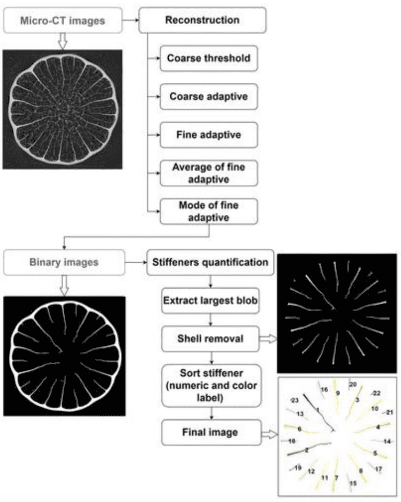
Fig. 1. Flow chart of stiffeners quantification via Matlab image processing including a gray-scale micro-CT of an African Porcupine Quill, as well as reconstructed (virtual) cross sections of the spine (Tee et al., 2022).

Building a model for the stiffeners requires calculating the porosity of the various spines and quills measured from the micro-CT images. The porosity was calculated for 4 samples using the volume of the segmented background (air) within the quill to the segmented sample, as seen in Figure 2 (Tee et al., 2022). Three different methods were used for this calculation to help identify which method works best.

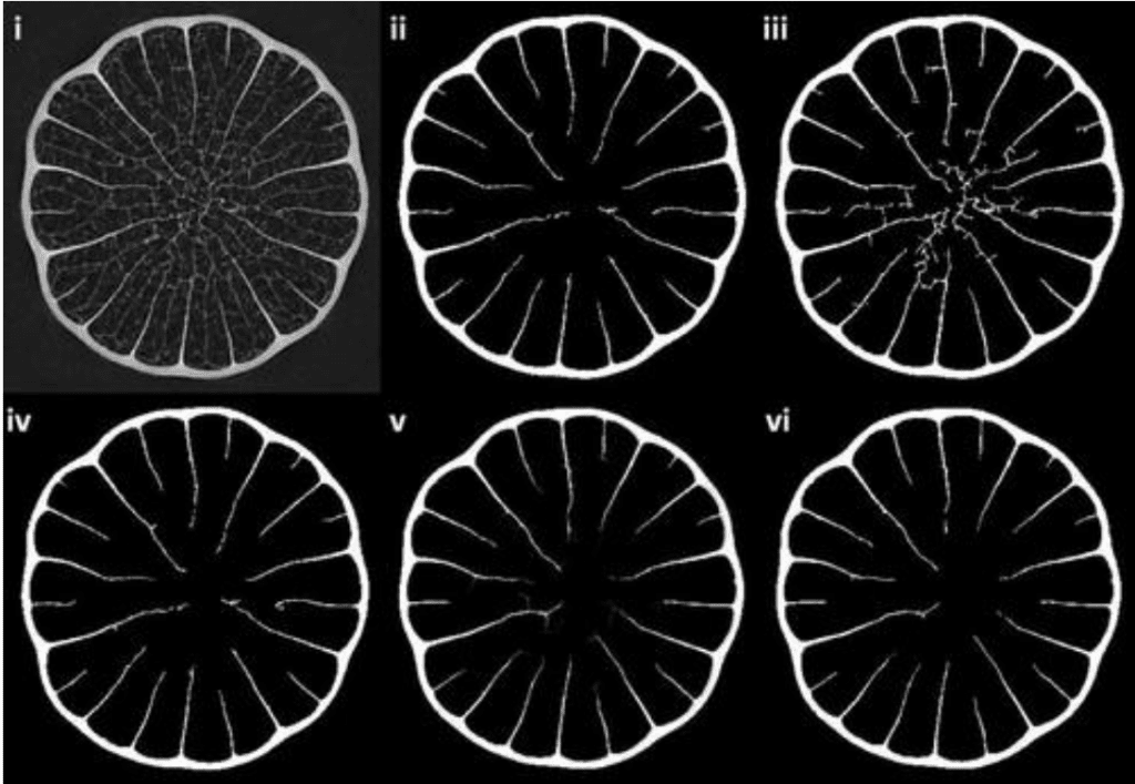
Fig. 2. Comparisons of segmentation modes (Tee et al., 2022). (i) Original grayscale image, (ii) coarse threshold, (iii) coarse adaptive (with a  gray-scale gradient steepness sensitivity value of 0.3), (iv) fine adaptive (with a sensitivity value of 0.05), (v) average of fine adaptive and (vi) mode of fine adaptive.

As noted in Figure 1, various segmentation modes were used before the µCT image could be adapted for binary usage. The various segmentation modes and results are described in Figure 2 (Tee et al., 2022). Different extraction modes already result in visibly different outputs. Additionally, the threshold level prescribed to a specific segmentation mode may also result in a broad range of results. This is why extensive model design and testing is essential to ensure that the region of interest can be specifically isolated in the design of a specific model. 

Interestingly to note is that as the quills grow in size, we also see more stiffeners present (Tee et al., 2022). As seen in Figure 3, the quills were modeled and appeared to present a recurring pattern that could potentially help with mechanical loading. The stiffener length seems to vary such that there is always a long stiffener close to a shorter one.

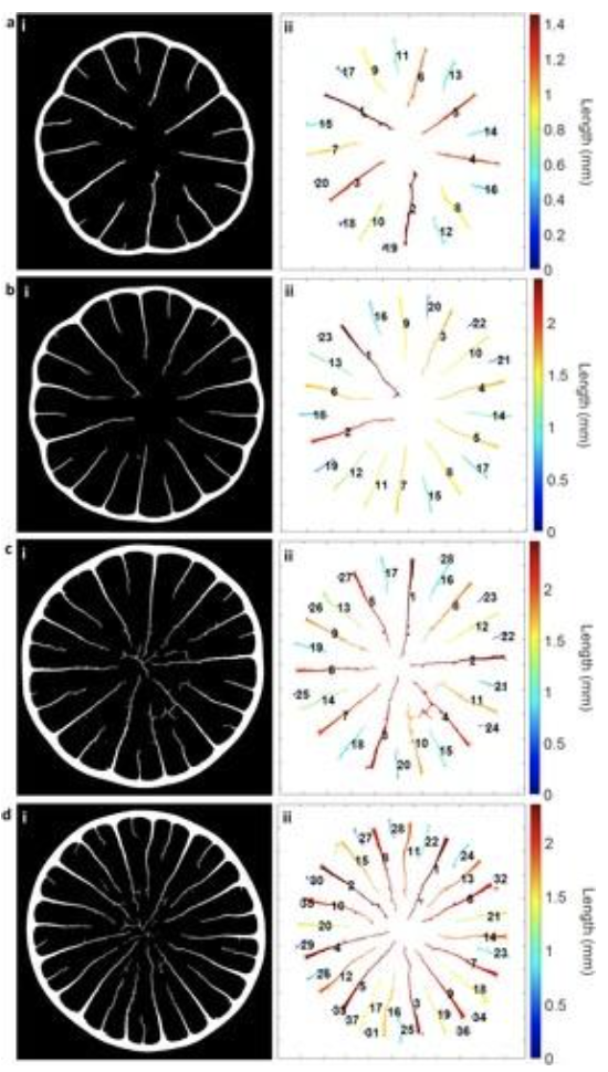
Fig. 3. Quill stiffeners quantification, numerical and color-coded from the longest to the shortest length: (a) Q1, (b) Q2, (c) Q3 and (d) Q4 (Tee et al., 2022).

To further investigate the porosity of these quills and find new ways to quantify them, the three methods were implemented, yielding various results as described in Figure 4.

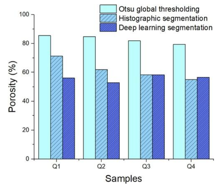
Fig. 4. Porosity comparison between different segmentation methods. Otsu global thresholding, histographic segmentation, and deep learning segmentation (Tee et al., 2022).

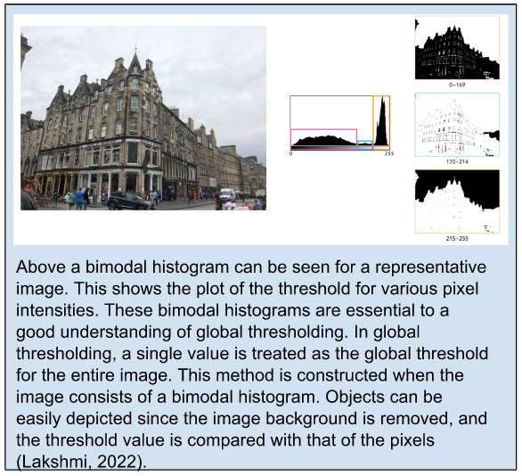
Otsu global thresholding is one of the most common methods used for separating foreground pixels from the background, generally called thresholding (Otsu et al., 1979). This is a variance-based technique that finds the threshold value when the weighted variance between the foreground and the background is the least. To better understand this, we need to look at the equation for finding within-class variance at any threshold, t, which is outlined in Equation 1.

\begin{equation}
\sigma^2(t)=\omega_{bg}(t)\sigma^2_{bg}(t)+\omega_{fg}(t)\sigma_{fg}(t)
\end{equation}

ω_bg(t) represents the probability of the number of pixels for each class in the background at a given threshold t. ω_fg(t) represents the probability of the number of pixels for each class in the foreground at a given threshold t. σ² represents the variance of the color values.

\begin{equation}
\sigma^2=\frac{\sum(xi-x)^2}{N}
\end{equation}

The variance value can be calculated using Equation 2. It is important to note that we are counting the number of pixels. This variance has to be calculated for both the foreground, and the background. Various scripts using diverse computational languages like Python and Matlab have been written to adapt these methods for computation. Another more complex method seen in Figure 4 is deep learning segmentation. This method requires a much more rigorous mathematical and computational background to understand. In short, deep learning segmentation takes advantage of the learning process developed for artificial intelligence, allowing images to be partitioned into multiple segments or objects (Szeliski, 2011). There are broad applications of deep learning image segmentation, from autonomous cars to medical imaging and diagnostics. Concerning porcupine spines, the three methods used result in different images, so it is clear that different methods yield different porosity results (Figure 5).

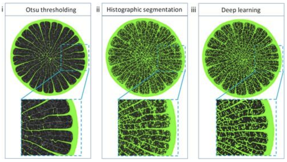
Fig. 5. Image segmentation of porcupine quill (Q4) using (i) Otsu global thresholding, (ii) histographic segmentation, and (iii) deep learning segmentation (Tee et al., 2022).

Even between the different computational methods used to characterize these spines, significant differences can be seen. Differences, when applied to other engineering applications, could potentially be extremely important. Deep learning should be used for a model where picking up on the finest of details is important. However, Otsu thresholding could serve as a fast analytical solution, giving us a reasonably high level of accuracy without using significant resources – where the image quality, and object complexity allow it. 

Researchers generated a volume thickness map to further characterize these reconstructed µCT images to understand local geometric variation across samples (Tee et al., 2022). This method was used to understand the relative thickness of stiffeners better as they elongate towards the center of the spine (Figure 6).

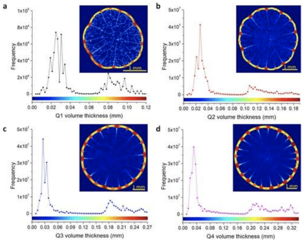
Fig. 6. Volume thickness map of porcupine quill samples and the respective frequency graph: (a) Q1, (b) Q2, (c) Q3 and (d) Q4 (Colour legend above x-axis represents the thickness of the porcupine quill in the respective inset) (Tee et al., 2022).

The thickest region of the stiffeners appears at the junction with the shell, which is logical since we would like our structure to have the most stability at its base. From a load-bearing perspective, it makes sense to have thicker structures that can bear more leads closer to the exterior. This results in better absorption of stress than if the thickest structures were in the middle, resulting in a frail exterior with a strong interior structure. Mathematically derived models like the following are useful since they allow engineers to further understand the basic mechanics that give strength to various spinous structures. These basic principles can then be adapted and modified for general usage, like beams and bridges, to design sturdy but malleable tissue regeneration scaffolds. 

Modeling porcupine spines present various engineering applications in different domains. Ghazlan et al. (2021) describes designing a cellular structure for mitigating the effect of loadings based on the porosity of porcupine spines. The mathematical models that allow researchers to unravel the mysteries of the natural world endow them with the potential to purposefully apply these discoveries to build better cellular grafts, load-bearing columns, or even bridges. A model made to characterize how divergent hair growth in rodents becomes a spine describes this (Gonçalves et al., 2018).

Cacti spines and Laplace pressure

Cacti, like other plants, need water to survive. The spines, therefore, have an essential function. They gather droplets of water from the air and guide them to the base of the spine. Different models of cactus spines have been designed to try to understand how the geometry of the spine allows the droplet to slide from the tip of the spine to its end. Many studies propose a conical model with a smooth circular cross-section of the spine (Figure 8). However, cactus spines present micro ridges, very small and narrow striations, as shown in Figure 7 (Guo et al., 2021).

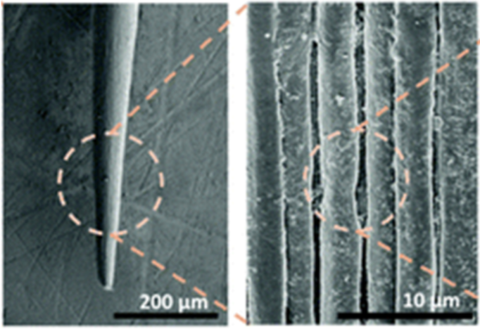
Fig. 7. Microridges are present on the surface of a cactus spine (Guo et al., 2021).

Models with noncircular cross-sections have been designed to mimic the uneven structure due to the micro ridges present on the conical surface of the spine. An algorithm has been developed to evaluate and compare the droplet movement on different spines models. Dissipative particle dynamics have been used for modeling. Simulations were performed on spines with the same base radius (Guo et al., 2021).

Fig. 8. Three different cross-sections of spines were tested. The tri-concave and penta-concave are examples of pyramidal cross-sections (Guo et al., 2021).

The cactus spine uses self-propelled directional liquid transport to have the droplet go from the tip to the base of the spine. The force that drives the droplet against gravity is called the Laplace pressure gradient and is generated by the curvature gradient. There is a difference between the pressure inside and outside the droplet. The droplet will move toward a higher radius to decrease this pressure. In all models, the droplet, initially at the tip, moves to the structure’s base (Guo et al., 2021).

The Laplace pressure difference (Δp) between the inside and outside of the droplet is given by Equation 3 and shown in Figure 9.

\begin{equation}
\Delta p=2\gamma(\frac{1}{r_1}-\frac{1}{r_2})
\end{equation}

Where r₁ and r₂ are the radii of the spine on each side of the droplet, and is the surface tension.

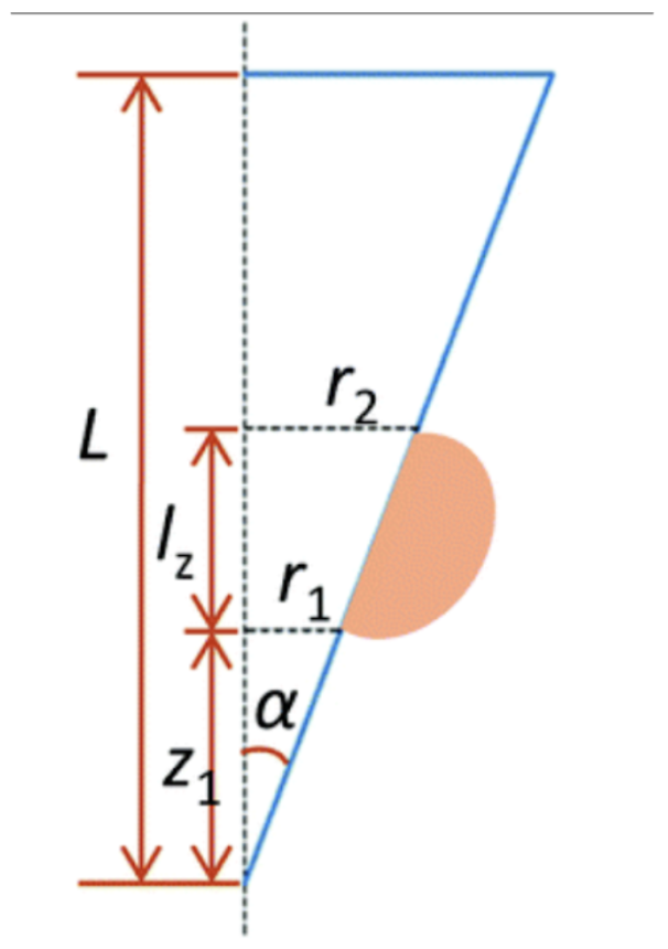
Fig. 9. Schematic diagram of a conical model with circular cross-sections (Guo et al., 2021). Looking at this schematic, another equality for p can be derived.

\begin{equation}
\tan(\alpha)=\frac{r_1}{z_1}=\frac{r_2}{z_2}=\frac{r_b}{L}\\ r_2=\frac{r_b(l_z+z_1)}{L},r_1=\frac{r_bz_1}{L}\\\Delta p=\frac{2\gamma L}{r_b}(\frac{1}{z_1}-\frac{1}{z_1+l_z}
\end{equation}

Where γ is the surface tension, L is the length of the spine, r_b the radius of the base of the spine and z₁ the vertical distance between the tip of the spine and the droplet. From this equation, we can notice that the Laplace pressure difference is inversely proportional to the radius, which means that the droplet will move more easily if the radius is small. Moreover, high surface tension and a great length increase the Laplace pressure difference. For the model with a concave cross-section, however, this formula differs. The Laplace pressure (Δp) will be given by the sum of the Laplace pressure difference for a cone and the individual concave surfaces, as shown in Equation 5 (Guo et al., 2021). The equation is based on the schematic of Figure 10.

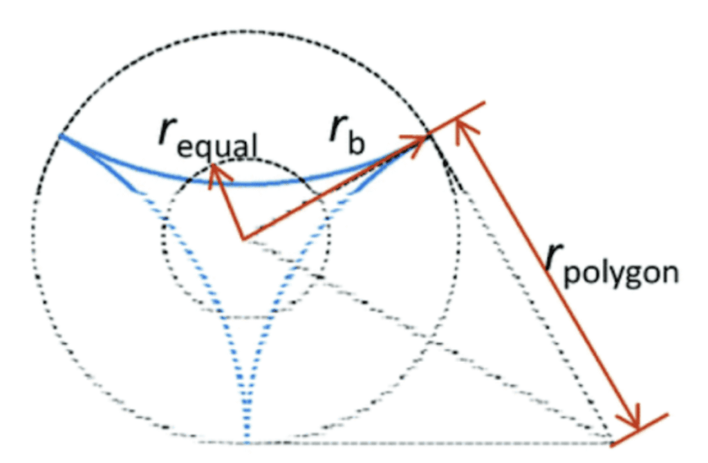
Fig. 10. Schematic diagram of a tri-concave cross-section (Guo et al., 2021).

\begin{equation}
\Delta p=2\gamma(\frac{1}{r_{1equal}}-\frac{1}{r_{2equal}})+2\gamma(\frac{1}{r_{1polygon}}-\frac{1}{r_{2polygon}})
\end{equation}

Where r_equal is the radius of the circle equivalent to the pyramidal cross-section, r_polygonis the half side length of the polygon circumscribed about the base circle and γ is the surface tension. This pressure also depends on the number of concave faces. 

The simulations show that the moving velocity and the distance traveled vary with the model (Figure 11). The tri-concave cross-section has a greater velocity and moving distance than the circular cross-section (Guo et al., 2021).

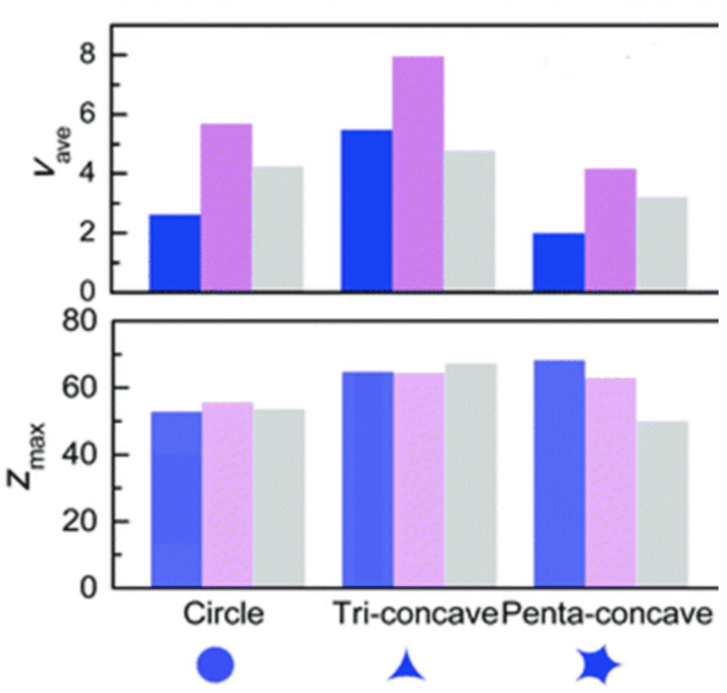
Fig. 11. Average velocity (V_ave) and maximum distance (Z_max) of the droplet under various cross-sections and radii of droplets (Guo et al., 2021).

The two modes of annular and side motion, explain this difference in velocity and distance (Figure 12). In the model with the circular cross-section, the droplet has an annular motion, which means it first moves around the cone before going to the side. This results in an increased contact area and friction force. For the second model, the droplet moves laterally on the spine. This model, which reflects the micro ridges in the spine, would facilitate the movement of the droplet because the shape of concave sides leads to a smaller contact area. This decreases the resistance to motion. Therefore, the micro ridges reduce the base radius and contact area, which increases the driving force (Guo et al., 2021).

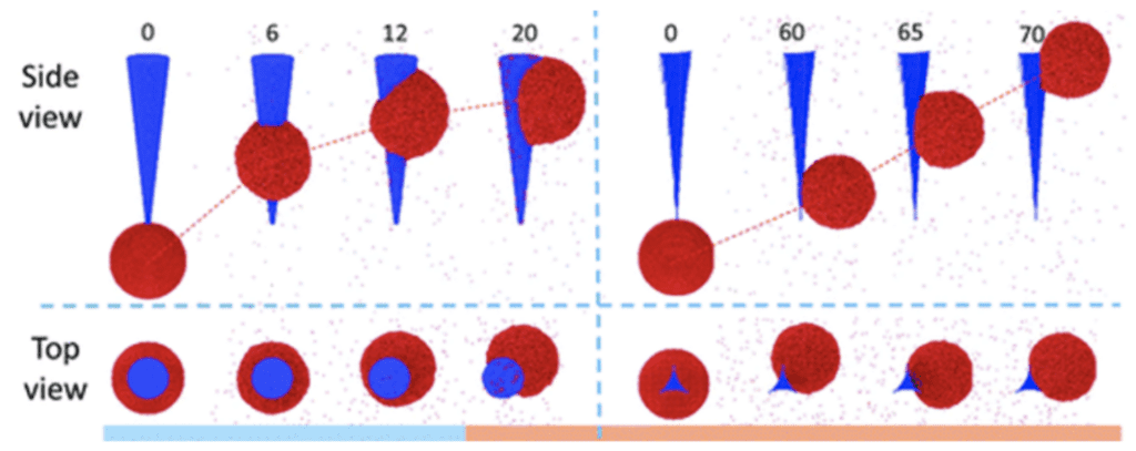
 Fig. 12. Annular (left) and side (right) motion of the droplet (Guo et al., 2021).

Several factors influence the motion of the droplet along the spine. Increasing the conical angle results in a smaller average velocity of the circular cone. In the case of the tri-concave fiber, however, the distance is reduced. This is explained by the angle increase that leads to an increase in the radius. As can be seen in Equation 5, a larger radius leads to a smaller Laplace pressure difference. Thus, the driving force is reduced. The tri-concave shape, however, produces a smaller change in the base radius, resulting in a smaller velocity change than for the circular cone (Guo et al., 2021).

Water has a high surface tension compared to other liquids. Indeed, the high cohesive forces between the water molecules allow them to stay together and resist external forces. As shown in the model, the concave shape of the lateral surface of micro ridges also gathers the water molecules, enabling side motion. When the surface tension is greater than 11.17, however, the droplet cannot move along the spine and is detached from the surface (Figure 13) (Guo et al., 2021).

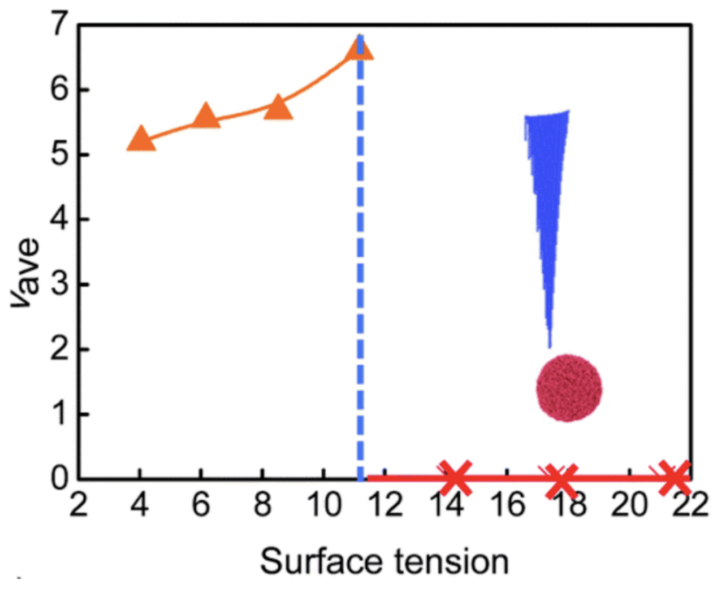
Fig. 13.  Average velocity as a function of the surface tension. Droplet detaches from the surface when tension exceeds 11.17 (Guo et al., 2021).

The micro-ridges in cactus spines probably maximize the ability to transport water droplets (Figure 14). Other plants have developed similar structures to facilitate water collection. The Namib grass Stipagrostis sabulicola, for example, has developed grooves within the surface to conduct the water towards the plant base (Roth-Nebelsick et al., 2012). A better understanding of those structures could help in the development of microfluidics.

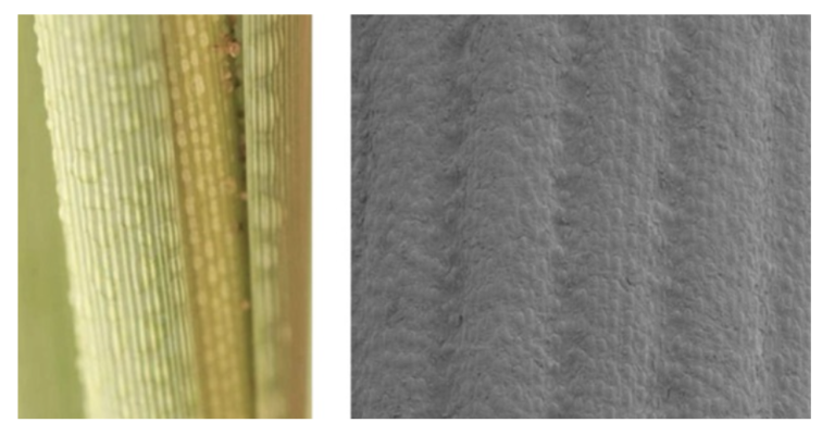
Fig. 14. The micro-ridges of cacti spines (Roth-Nebelsick et al., 2012).

Spines of acacia and their defense against ungulates

In Africa, there is an abundance of ungulates that consume plants.  Ungulates are large-hooved mammals, forming a significant population of herbivores on the continent.  Giraffes, goats, zebras, impalas, and kudus are all considered ungulates.  Plant spines are an effective defense against herbivores of plant species. Tropical American plants are known to possess spines, while trees in Australia lack spines on many taller plants as they lack herbivore foraging at these heights. Acacias are drought-resistant trees abundant in Australia and Africa (Figure 15).  There are over 160 tree species of Acacia, and many contain spines that restrict herbivore access to their leaflets (Figure 16)(Petruzzello, 2020).  In South Africa, species of Acacia and their defensive spines were studied with kudus (Tragelaphus strepsiceros) and impalas (Aepceros melampus) (Cooper & Owen-Smith, 1986).  Kudus and impalas were studied within a nature reserve of 213 hectares, and over two years, their grazing of spiny Acacia species was compared to non-spiny plant species (Figure 17).

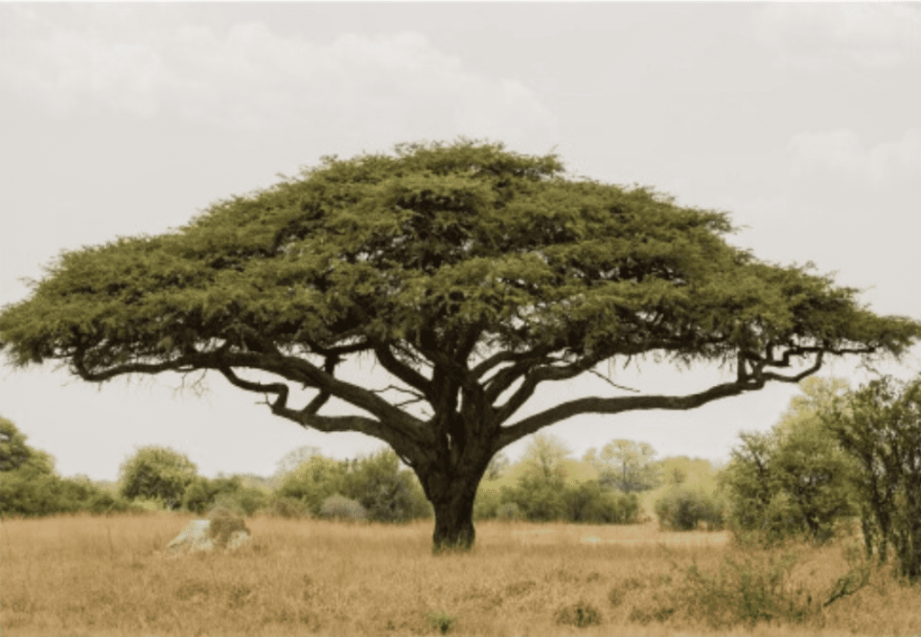
Fig. 15. Acacia tortilis is the predominant foliage species in East Africa (Townsend & Barton, 2018).

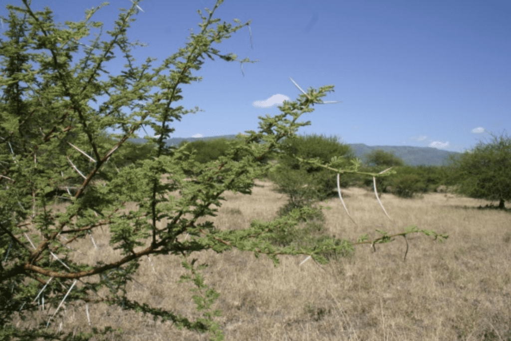
Fig. 16. The white spines of juvenile Acacia tortilis defend against herbivore grazing (Roland, 2017).

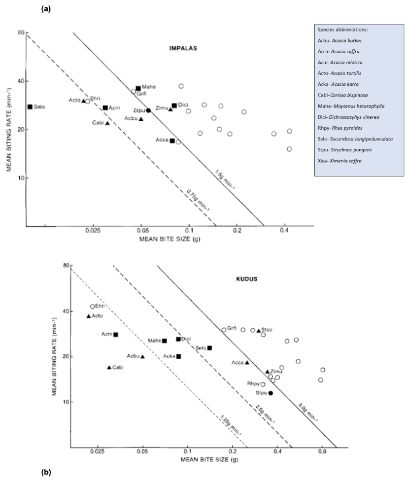
Fig. 17. The mean biting rate per miniature is plotted on a log-log scale with the mean bite size by dry mass.  Solid triangles represent the plants whose spines are curved, and solid squares represent plants whose spines are straight.  Species with spines are solid circles, and open circles indicate spineless species, some of which are unnamed. Solid and dashed lines show slopes of the indicated food intakes in g/min.  (a) shows the mean biting rate of Kudus, while (b) is the mean biting rate of impalas (Cooper & Owen-Smith, 1986).

Based on the graphs in Figure 17, the spineless species increased the rates of their bites as their bite sizes decreased. Spineless species allowed both Kudus and impalas to have larger bite sizes. Spines did not significantly impact the mean biting rate. However, there was a significant disparity between the bite sizes, with spines reducing the foraging bite size.  Furthermore, impalas and kudus could not increase their consumption rates to compensate for the lower bite sizes. Kudus and Impalas require 1.5 g/min (represented by a solid line in Figure 17(a) to achieve a daily food intake of 2-2.5% body mass (Cooper & Owen-Smith, 1986). In Figure 17(a), spineless plants allow impalas to exceed this consumption rate. Acacia species were consumed closer to 0.75g/min; their spines hindered the grazing from impalas. The most unfavorable species for consumption were the Acacias, with their hooked spines, kudus consumed these species only at a rate of 1 g/min.  

Thorns have two defensive mechanisms. They can penetrate the soft tissues in the mouths of animals and restrict the bite sizes of herbivores. Thorns on Acacias that have been browsed or consumed are longer than plants that have not experienced grazing.  Thorns on lower branches were 26-27% longer than thorns of a similar height on unbrowsed plants (Figure 18). Thorns of browsed plants were also 36-44% longer than branches above goats’ reach.  In a study of Acacia in Kenya (Young, 1987), where goats and their consumption of branches were examined, thorn length was calculated. The goat population interacted with the Acacia for over 30 years.  The control sample of Acacia did not experience any browsing pressure over time.

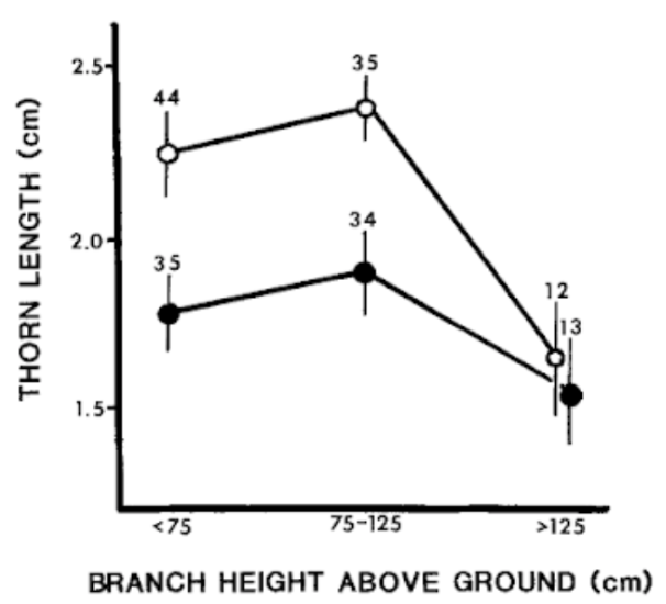
Fig. 18. The mean thorn length (cm) of thorns on Acacia depranolobium trees. The solid circles are of unbrowsed trees, and the browsed trees are empty circles. Vertical lines indicate standard error (Young, 1987).

Grazing of branches on Acacia induced morphological defenses of the plant, producing longer spines. Specifically, goats can consume the shoots of Acacia by pruning the tips and leaves using their molars or by picking the leaves and clusters with their tongues.  These cropping methods and the spines’ presence influence the feeding rate (Figure 19). In Tanzania, Acacia tortilis were examined along with the feeding rate of goats.  Mature Acacia tortilis lack spines, while juvenile Acacia tortilis contain spines and can dedicate up to 10% of their biomass to the production of spines. The biomass consumed was the difference between the expected mass of the twig and the actual remaining mass. Both methods of foraging, pruning, and picking of leaves by the goats were calculated. The fresh mass ratio of leaves to twigs was 0.53:0.47, which was used in the calculations of equations 6 and 7 (Gowda, 1996). The biomass of the spiny branches picked by the goats was evaluated with the following equations:

\begin{equation}
Biomass\;picked=w_3/0.47-w_2
\end{equation}

The remaining twig mass is w3, and w2 is the mass of the remaining twigs and leaves after goat grazing. The pruned biomass was the mass picked subtracted from the mass lost.

\begin{equation}
Biomass\:pruned=(w_1-w_3/0.47)
\end{equation}

In equation 6, w1 is the initial biomass of the branches.

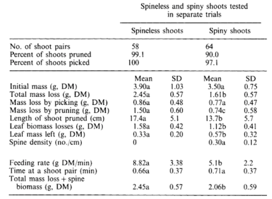
Fig. 19. Spineless and spiny Acacia tortilis were studied under the grazing of goats.  Using Equations 1 and 2, the dry masses (DM) in grams (g) lost by pruning and picking were calculated. The feeding rate was calculated from the biomass loss divided by the feeding interval (Gowda, 1996).

Increases in spine density affect the feeding rates of goats. There is a lower feeding rate and twig biomass is removed as spine density increases (Figure 20). As spine density increases, goats change from foraging by pruning shoot tips to picking leaves. The feeding rate is also increased in spineless shoots compared to spring shoots.

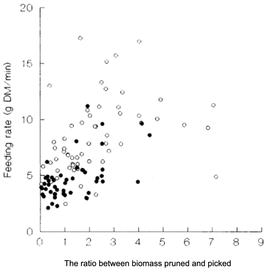
Fig. 20. An increase in remaining biomass that can be pruned compared to what can be picked by goats leads to an increase in feeding rate (DM g/min). The solid circles are spiny shoots, and the open circles are spineless shoots (Gowda, 1996).

The spines of various species in the Acacia species reduce the feeding rates of ungulates such as impala, kudus, and goats.  As there is limited vegetation in the savannah and regions of study in Kenya and South Africa, Acacia have utilized defensive morphology, which deters foraging. The correlation between increased spined and decreased feeding rates has been modeled using log-log scales (Figure 20), along with data on spineless vegetation and the grazing of these species. 

Voronoi patterns in spine tubercles of sea urchins

Nature has shown mass-produced yet mind-blowing structures that minimize required resources. One famous example is the slime mold experiment that grew a vein network similar to the human-engineered Tokyo subway system. Another less renowned example is the intricate pattern found in the sea urchin spine’s tubercle (Figure 21), or the spine attachment site.

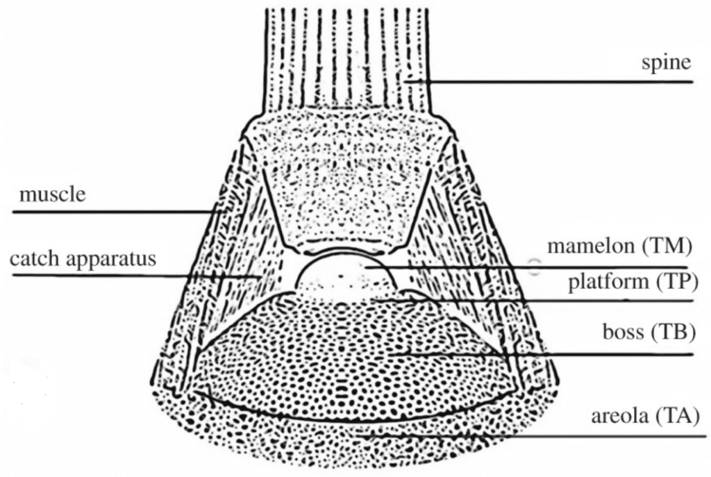
Fig. 21. Model of a spine belonging to the Paracentrotus Lividus, its tubercle, and other soft tissues connecting the whole. The tubercle is composed of the tubercle areola (TA), the tubercle platform (TP), the tubercle mamelon (TM), and the tubercle boss (TB) (Perricone et al., 2022).

The Voronoi model can mimic the  specific pattern of the spine tubercle. In short, it is a method to divide a two-dimensional or three-dimensional space into multiple polygons referred to as Voronoi cells. By placing points in predetermined positions, each point will become the seed of a Voronoi cell. Finally, sides are drawn by placing them equidistant to the two nearest Voronoi seeds (Figure 22) (Sehat et al., 2021).

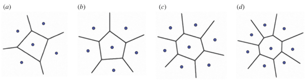
Fig. 22. Model of the Voronoi model with (a) 5, (b) 6, (c) 7 and (d) 8 seeds. The center Voronoi cell in each example has an equal number of sides as neighbor seeds. Notice how each side of the central polygon is at an equal distance from the central seed and the next closest seed (Perricone et al., 2022).

The stability of a structure following the Voronoi model is proportional to several factors like the generality of the polygons, the shape of the cells, the number of cells, the cell distribution, and the wall thickness. The most performant arrangements can often handle a large amount of stress thanks to their optimized stress-transferring capacity and  lightness. It is easy to see when looking at other durable structures like the hexagonal beehives or the peculiar shapes on the turtle shell. As such, the same can probably be inferred for the sea urchin’s tubercle. 

To turn the porous tubercle into an array of polygons, scientists had to transform the structure with varying wall thickness into a group of lines and nodes (Figure 23). As a result, the following analysis of the tubercle’s stability will not consider the wall thickness and the generality of wall thickness.

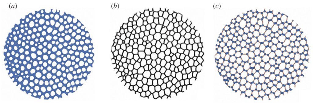
Fig. 23. Process of polygonization of the Paracentrotus Lividus tubercle boss cross-section. Image (a) was taken by SEM micrograph binarization. This means that there are only two categories of “space”, being empty space in white and filled space in blue, regardless of the original density of the crystal calcite at that original position. Image (b) is the polygonized alteration of image (a), while image (c) shows the line and nodes of each polygon seen in image (b) (Perricone et al., 2022).

Additionally, they also had to create a control Voronoi model, or the ideal structure. This one should have the same number of seeds at the same positions as the experimental Voronoi model (Figure 24). A second model was created by identifying all the pores in the tubercle boss, then selecting the centroid of each pore as the seed of the Voronoi cell (Figure 25).

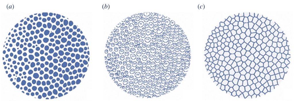
Fig. 24. Process of generating the ideal Voronoi model of the Paracentrotus Lividus tubercle boss. Image (a) was created by SEM micrograph binarization. The blue spaces represent the pores, while the white spaces represent the walls. Image (b) identifies all the pores as a 2D shape with an ID number, then image (c) illustrates the ideal Voronoi model by computing the centroid of each shape as a seed, then generating the structure based on the conditions of the model (Perricone et al., 2022).

Finally, the two models were superposed to visually show the differences between the actual tubercle and the ideal tubercle (Figure 26).

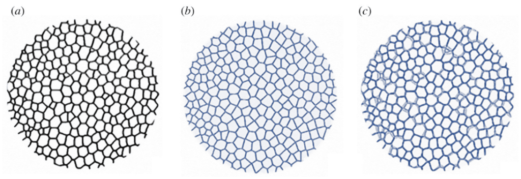
Fig. 25. Superposition of the actual tubercle Voronoi model and the ideal tubercle Voronoi model. Image (a) is the experimental tubercle. Image (b) is the ideal tubercle. Image (c) is the superposition of both image (a) and (b) (Perricone et al., 2022).

After analysis, it has been revealed that the sea urchin tubercle boss is about 82% identical to the ideal Voronoi model (Figure 26), similar to the accuracy of a hexagonal honeycomb. In addition, there is a wide variety of polygons ranging from the triangle to the decagon, although the largest portion of polygons is composed of hexagons (Figure 27).

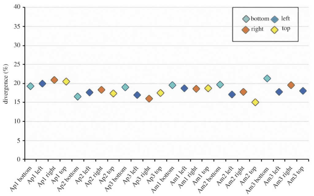
Fig. 26. Divergence trend between the ideal Voronoi model of the tubercle boss and the actual tubercle boss in multiple regions. There were three different Paracentrotus Lividus spines, identified by the corresponding index at the end of each category. There is a top, bottom, left, and right region for each tubercle boss, so they were all measured separately. Finally, there are Apical plates (Ap), which correspond to the youngest and smallest plates on the sea urchin, and the Ambital plates (Am), which correspond to the older and bigger plates (Perricone et al., 2022).

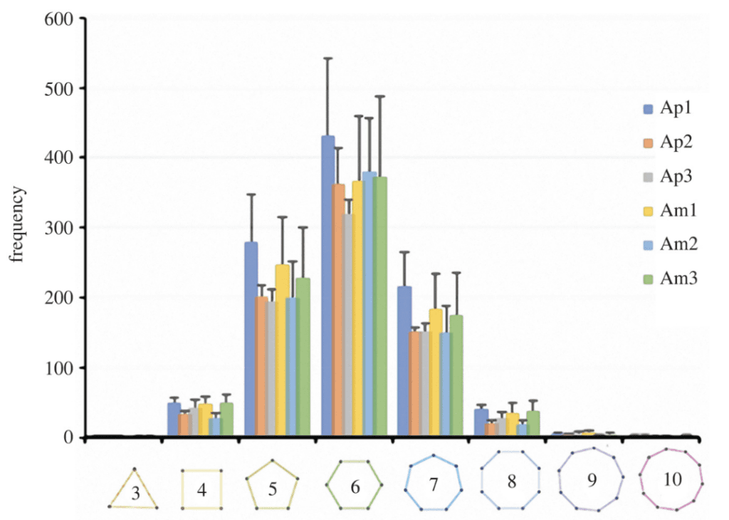
Fig. 27. Histogram of the number of neighbor seeds or sides for all Voronoi cells in all regions and spines. Notice the general bell curve of the histogram closely favoring the middle. It is also hypothesized that there is a wide range of polygons due to constraints during cell growth and proliferation, in patterns, and morphogenesis (Perricone et al., 2022).

Similarly to many other natural constructions, the sea urchin’s tubercle also takes advantage of the hexagonal shape. This in itself provides several advantages in terms of stability and resources. Firstly, suppose one were to attempt to fill a two or three-dimensional space with simple polygons without giving rise to gaps or overlaps between polygons. In that case, it could only be achieved using triangular, quadrilateral, or hexagonal polygons (Perricone et al., 2022). Moreover, hexagonal shapes can grid space with the least possible perimeter. Indeed, this is in accordance with the fact that the sea urchin can produce volumes composed of crystal calcite with scarce resources while maintaining a strong and durable material. Secondly, the particular property of a structure that follows a Voronoi model is that if an external force is applied at a specific site, the distortion will spread throughout the entire grid. Every polygon will be slightly distorted, as opposed to concentrating all the force onto a single polygon (Reem, 2011). Consequently, the tubercle can handle great stress if the spine is compressed onto itself, as the stress is redistributed and spread out through all the polygons, and no fracture occurs (Perricone et al., 2022). 

In light of the properties mentioned above, there is a specific way for the sea urchin to take advantage of the durability of the tubercle when contracting its spine muscles. There is a thick system of spine muscles between the spine and the areola (Figure 21). If it were contracted in a specific direction, the spine could be pulled in any direction on the ball-and-socket joint composed of the base of the spine and the mamelon (Figure 21). This is useful for moving the spine back and forth when the sea urchin displaces itself. As such, it is easy to see that doing this repetitive back-and-forth motion is held all together thanks to the structural stability of the tubercle holding the system afloat(Perricone et al., 2022). If the sea urchin is under fire from a predator, it can quickly contract all muscles in all directions to clamp the spine, making it extremely rigid. Measurements have found that the muscles can exert tensile stresses up to 40 MPa in these instances, also supported by the highly efficient structure of the tubercle (Perricone et al., 2022).

In conclusion, many properties of the sea urchin’s organically produced crystal calcite are revealed thanks to its specific pattern. Indeed, the Voronoi model accurately describes its pores, and yields a highly spacious yet resource-efficient volume capable of handling large amounts of stress. This follows observations made before the discovery of this pattern, such as the lightness and durability of the material. Most importantly, this shows how living beings’ disorderly and chaotic natures often follow strict mathematical principles and functions.

Conclusion

Mathematics allows for the aided interpretation of natural behaviors and phenomena. The diversity of spines can be further appreciated through equations and modeling. Porcupine spines and their structure can be analyzed with micro-CT scans, and Otsu thresholding is used to separate the pixelated images. More advanced and costly methods, like Deep Learning Segmentation, can also be applied to characterize these spines. Modeling software such as Matlab and various other computational programs and languages allow for further analysis. The Laplace equation can be used to understand the pressure experienced by water droplets on a cactus spine. The mathematical relationship between biomass consumed and spine length has aided researchers in discovering the impact of Acacia spines on the feeding of herbivores of the region. Finally, Voronoi models are employed by researchers to describe the spinal structure of sea urchins.  With abundant connections to mathematics, spines exemplify how the pandemonium of nature encourages the extension of engineering principles. 

References

Cooper, S. M., & Owen-Smith, N. (1986). Effects of plant spinescence on large mammalian herbivores. Oecologia, 68(3), 446–455. https://doi.org/10.1007/BF01036753

Ghazlan, A., Ngo, T., Le, V. T., Nguyen, T., Linforth, S., Remennikov, A., & Whittaker, A. (2021). A bio-mimetic cellular structure for mitigating the effects of impulsive loadings – A numerical study. Journal of Sandwich Structures & Materials, 23(6), 1929-1955. https://doi.org/10.1177/1099636220908581 

Gonçalves, G. L., Maestri, R., Moreira, G. R. P., Jacobi, M. A. M., Freitas, T. R. O., & Hoekstra, H. E. (2018). Divergent genetic mechanism leads to spiny hair in rodents. PLOS ONE, 13(8), e0202219. https://doi.org/10.1371/journal.pone.0202219 

Gowda, J. H. (1996). Spines of acacia tortilis: What do they defend and how? Oikos (Copenhagen, Denmark), 77(2), 279. https://doi.org/10.2307/3546066

Guo, L., Kumar, S., Yang, M., Tang, G., & Liu, Z. (2021). Role of the microridges on cactus spines. Nanoscale, 14(2), 525–533. https://doi.org/10.1039/d1nr05906h

Lakshmi, J. V. N. 5 – Deep learning on medical image analysis on COVID-19 x-ray dataset using an X-Net architecture. In Deep Learning for Medical Applications with Unique Data, Gupta, D., Kose, U., Khanna, A., Balas, V. E. Eds.; Academic Press, 2022; pp 71-106.

Otsu, N. (1979). A Threshold Selection Method from Gray-Level Histograms. IEEE Transactions on Systems, Man, and Cybernetics, 9(1), 62-66. https://doi.org/10.1109/TSMC.1979.4310076 

Perricone V., Grun B. T., Rendina F., Marmo F., Carnevali C. M. D., Kowalewski M., Facchini A., Stefano D. M., Santella L., Langella C., Micheletti A. (2022). Hexagonal Voronoi Pattern Detected in the Microstructural Design of the Echinoid Skeleton. Journal of the Royal Society. 19. 193. https://doi.org/10.1098/rsif.2022.0226

Petruzzello, M. (2020). Acacia. In Encyclopedia Britannica. https://www.britannica.com/plant/acacia

Reedy, C. L., & Reedy, C. L. (2022). High-resolution micro-CT with 3D image analysis for porosity characterization of historic bricks. Heritage Science, 10(1), 83. https://doi.org/10.1186/s40494-022-00723-4 

Reem D. (2011). The Geometric Stability of Voronoi Diagrams with Respect to Small Changes of the Sites. ACM Digital Library. 254-263. https://doi.org/10.1145/1998196.1998234

Roland, W. A. (2017). Acacia tortilis ssp. heteracantha. Acacia-world.net.http://www.acacia-world.net/index.php/africa-me/south-africa/acacia-tortilis-ssp-heteracantha/

Roth-Nebelsick, A., Ebner, M., Miranda, T., Gottschalk, V., Voigt, D., Gorb, S., Stegmaier, T., Sarsour, J., Linke, M., & Konrad, W. (2012). Leaf surface structures enable the endemic Namib desert grass Stipagrostis sabulicola to irrigate itself with fog water. Journal of the Royal Society, Interface, 9(73), 1965–1974. https://doi.org/10.1098/rsif.2011.0847

Sehat S., Khatami A. (2021). Parametric study on application of Voronoi patterns in design of 2-D beams. Sage Journals. 24. 11. https://doi.org/10.1177/1369433221999740

Song, W., Mu, Z., Zhang, Z., Wang, Y., Hu, H., Ma, Z., Huang, L., Wang, Z., Zhang, B., Li, Y., Zhang, S., Li, B., Zhang, J., Niu, S., Han, Z., & Ren, L. (2021). Cross-Scale Biological Models of Species for Future Biomimetic Composite Design: A Review. Coatings, 11(11). https://mdpi-res.com/d_attachment/coatings/coatings-11-01297/article_deploy/coatings-11-01297-v2.pdf?version=1635487672 

Szeliski, R. (2011). Computer vision: algorithms and applications. Springer Nature. 

Tee, Y. L., Black, J. R., & Tran, P. (2022). Virtual characterisation of porcupine quills using X-ray micro-CT. Virtual and Physical Prototyping, 18(1), e2126377. https://doi.org/10.1080/17452759.2022.2126377 

Townsend, J. B., & Barton, S. (2018). The impact of ancient tree form on modern landscape preferences. Urban Forestry & Urban Greening, 34, 205-216. https://doi.org/10.1016/j.ufug.2018.06.004

Young, T. P. (1987). Increased thorn length in Acacia depranolobium -an induced response to browsing. Oecologia, 71(3), 436–438. https://doi.org/10.1007/BF00378718