Abstract

The animal kingdom encompasses all kinds of animals that collect their food supplies in unique ways. Consequently, by using mathematical language to describe these systems of behaviours, one can better understand and predict the way animals proceed during their food source search. This essay examines a few mathematical models describing this highly essential behaviour, foraging. Indeed, the Levy Processes, a model predicting the movement of foragers during patch selection, the Optimal Foraging Pattern, an efficiency description of how foraging animals capture randomly located prey, as well as the Marginal Value Theorem, a foraging efficiency model predicting when foragers should leave the patch, will all be investigated below. Furthermore, mathematical models describing the foraging activities for Honeybee flower selection and trail-laying Argentine ant pathway selection will also be studied. Lastly, 3 models studying the growth of population; one without external constraints, one with external constraints, and one with forager/prey interactions will be examined through the use of Stochastic ordinary differential equations. All in all, this paper concludes itself with the analysis of a variety of mathematical models, all while acknowledging the slight lack of complexity they all have; in fact, there are many additional occurring constraints that could be investigated to produce more elaborate models.

Introduction

The Optimal Foraging Theory, an ecological theory published in American Naturalist (MacArthur & Pianka, 1966), states that natural selection has favoured the survival of animals that forage in ways that maximize net energy intake per unit time (Lozano, 1998). The assumptions made by the Optimal Foraging Theory paved the way for the appearance of various mathematical models that predict the foraging patterns of animals. Given the complexity of the foraging decisions made by the animal species, most mathematical models have continuously been improved over the decades following its first formulation, through the incorporation of more parameters, such as traveling time, energy intake and energetic expenditure. Moreover, some mathematical models gave rise to more sophisticated mathematical theorems that further improve the accuracy of the foraging predictions.

Foraging is characterized by the interaction of foragers with food resources, be it autotroph or heterotroph. Thus, mathematical models are not only used to describe foraging patterns of animals, but also to describe the influence of forager activities on the forager population dynamics, as foraging affects the survival of the species. The essay first examines how mathematical models enhance our understanding of how animals make selective choices when foraging in patches, in ways that satisfy Optimal Foraging Theory. Secondly, the essay focuses on another interesting application of mathematical models in the context of foraging, namely the use of stochastic models to describe forager population dynamics.

Foraging Behaviours

Lévy Processes

Optimal foraging involves the tedious task of finding the suitable area to search for food items, identifying the targets despite many distractions, as well as estimating the time required to exploit the area. The assumption made by mathematical models is that food items are present in patches and foragers must travel between different patches and select patches to visit and/or leave (Charnov, 1976). Shlesinger and Klafter used a mathematical model, called Lévy Processes, to predict the movement of foragers during patch selection, specifically food patches that are sparse and randomly distributed (as cited in Viswanathan et al., 1999). Lévy Processes model a discrete sequence of steps and reorientation described as follows (Bella-Fernández et al., 2021):

P(l) = C \cdot l^{-u}

where length l is the vector representing steps separated by turning angles θ, and C, the normalizing constant. The parameter μ is in the range of 0 to 3. When the μ value exceeds 3, Lévy Processes turn into Brownian Motion, which can be considered as random walk. Examples of the Brownian Motion are the movement of dust in a room and the diffusion of calcium into bones (The Editors of Encyclopaedia Britannica, 2017). If, however, the μ value is less than 3, the forager is more likely to take long steps than does a random walker (LaScala-Gruenewald et al., 2019).

Research conducted by Viswanathan et al. (1999) suggested that each forager has a particular value of μ that optimizes its energetic gain per distance travelled. The research concluded that when foraging is considered nondestructive, meaning the food resource returns to its original state over time, the optimal μ value is approximately 2. On the other hand, if foraging is categorized as destructive, meaning when foraging results in food patches being completely depleted, the optimal μ value approaches 1 (LaScala-Gruenewald et al., 2019).

Furthermore, Viswanathan et al. (1999) developed the following foraging pattern that predicts foragers’ behaviour when prey is distributed randomly (Figure 1). The underlying principle is that foraging animals always try to maximize the efficiency of random search.

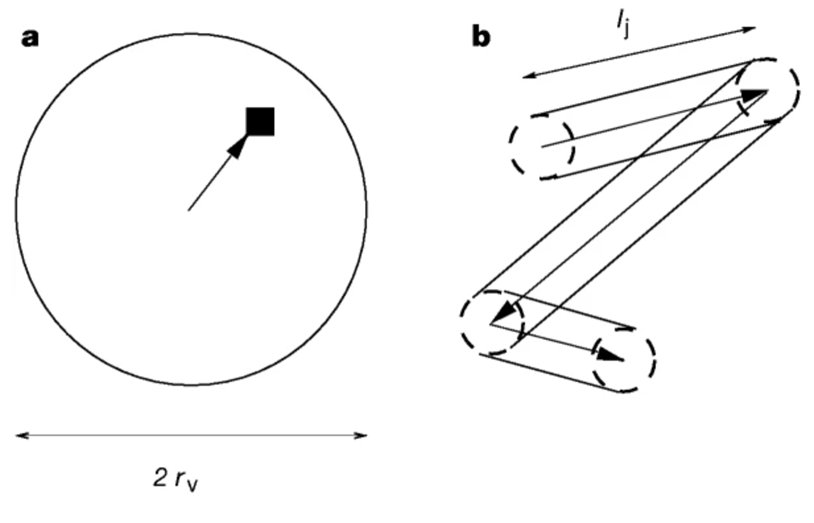
When the distance between the target and the forager is below a certain critical value r_v, the animal moves in a straight line to the target (Figure 1a). However, when the target is located beyond this distance r_v, no forager will be able to detect the target. Thus, if there is no target located within the radius r_v, the forager moves in a random direction and travels a random distance l_j from the probability distribution P(l_j) ∼ l-μ_j (Figure 1b). During its displacement, any target located within a distance r_v will be detected. If there is no target, the process is repeated by choosing a random distance and random direction.

Application of Marginal Value Theorem

Optimal Foraging Theory relies on the currency and the stopping rule. Currency is a way for foragers to measure energy intake (for example, the number of targeted food items), whereas the stopping rule affects the forager’s judgment of when it is best to leave the patch to exploit a new area (Charnov, 1976). Charnov (1976) proposed the Marginal Value Theorem (MVT), which describes the optimal stopping rule in animal foraging.

According to the MVT, the amount of currency, meaning the energy intake, is obtained by the function h(T), with an initial value of zero. The function h(T) demonstrates that the amount of currency h increases over time T, which implies that dh/dt < 0. However, as the amount of available resources decreases over time, the growth of currency decreases (d²h/dt² < 0).

An important assumption made by MVT is that the process of searching for food consumes energy, and that the resulting energy expense is proportional to the time spent foraging (T). Hence, a new function g(T) describing the net energy intake is defined, where Es x T corresponds to the energetic expenditure caused by foraging:

g(T) = h(t) - E_s \times T

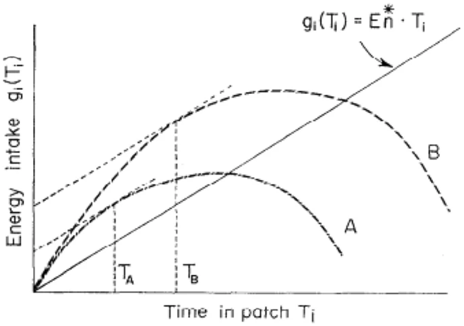
The MVT has been improved further, taking into consideration the cost of traveling E_t ⨯ T, where t is the total travel time. The finalized equation corresponding to the net energy intake rate (En) is defined, where 𝑃𝑖 is the proportion of the visited patches of type i (i = 1,2, …, k).

E_n (T_i) = \frac{\sum P_i \cdot g_i (T_i) - t \cdot E_t}{t + \sum P_i \cdot T_i}

The optimal time at which the forager should leave the patch in order to maximize currency is determined by plotting a line with a slope of E_n. The optimal currency gain rate is the value of gi when the line is tangent to the corresponding gi(Ti) curve (Figure 2). The T value at which the line and the curve intersect represents when the forager should leave the patch in question in order to maximize energy intake (LaScala-Gruenewald et al., 2019).

Mathematical Model of Ant Foraging Within Dynamic Environments

Ants do not navigate static environments, rather, they live in dynamically changing ones. Consequently, when foraging for food, the depletion of one food source can be matched by the appearance of others (Ramsch et al., 2012). Ant colonies have the ability to collectively choose the better of two available food sources (Reid et al., 2012). In order to make these decisions, they must be quick to adapt to changes in their foraging environment. In fact, mathematical models were developed to explain dynamic foraging behaviours and searching techniques of these very insects. These models were produced through the examination of foraging trail-laying Argentine ants that manage to determine the shortest paths within a complex dynamic maze (Ramsch et al., 2012). When in the maze, the simulated ants were either unfed on their way to their food source, or fed on root for the nest (Ramsch et al., 2012). The ant flow, number F(t) of unfed ants entering the maze at time t, is modeled by the following logistic equation:

\frac{dF(t)}{dt} = rF(t)(1 - \frac{F(t)}{K})

where r represents the recruitment rate, and K is the value of the flow at saturation (Vittori et al., 2006). Correspondingly, the flow of ants, at each second t, can be determined from integrating this previous equation, giving the following solution;

F(t) = \frac{F_{max}}{1 + (F_{max}/F_0 - 1)e^{-t/\tau}}

Where, F_max represents the maximum value of the flow, at saturation, and is a time constant based on the rate of recruitment (Vittori et al., 2006). At saturation the maximum number of foragers is reached, therefore it is related to the number of available ants for recruitment. In addition, a mathematical model is established for the branching choices made based on the pheromone trails left by these entering and exiting foraging ants. The Argentine ants use pheromones to navigate the dynamically changing environment; either depositing when foraging at the food source, or when exploring towards the nest (Ramsch et al., 2012). For instance, the selection between branches i and j for pheromone 𝛷_s would result with the probability p_s(i) of choosing i, denoted as the choice function that follows;

p_s(i) = \frac{(k_s + \Phi_s(i))^{\propto_s}}{(k_s + \Phi_s(i))^{\propto_s}+(k_s + \Phi_s(j))^{\propto_s}}

Where k_s represents the attraction of branches when disregarding pheromone s, and x_s being the non-linearity of the choice function. All in all, with mathematical language we can develop models that predict the behaviours of Argentine ants navigating through dynamic environments.

Mathematical Modeling for Flower Selection by Bees

There is a significant amount of literature on diets and food preferences of animals, but only few hypotheses and theories exist on how animals optimize their diets. Scientists have used mathematics to evaluate foraging strategies of animals which optimize the calorific benefits versus the energy consumed to reach the food source.

Keith Waddington and Larry Holden (1979) proposed a mathematical model for predicting the foraging activity of the honeybee (Apis mellifera) in an environment containing two varieties of flowers (Figure 3). The model predicts the strategy used by honeybees to maximize the caloric intake considering parameters such as the size and shape of the foraging area, flight time, and handling time.

The handling time begins when the bee lands on the flower and includes the time to extend the proboscis, to manipulate the floral mechanism and gain access to the nectar, to extract the liquid and to leave the flower. Surprisingly, the extraction time is the least expensive activity because most flowers visited by honeybees have very little quantities of nectar.

In the model, if the bee possesses sufficient information on the rewarding flowers and abilities to estimate distances, it will choose a foraging strategy which maximizes (Q), where Q = C/u, and (C) been the expected calorific reward and (u) the elapsed time between successive flower choices.

The equation of the elapsed time between flowers is u = (1/v)X + h which considers the mean flight speed of the bee (v), the distance to the chosen flower (X), and the handling time (h).

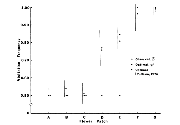
The validity of the model was confirmed by observing the behavior of 41 honeybees foraging at 7 flower patches, which do not differ in terms of proximity and which are made of just two varieties of flowers. Indeed, as shown in Figure 4, the model predicts the visitation frequency of bees foraging at seven patches in order to maximize the caloric intake and compares it to the observed frequency. Considering bees can make errors, such as not choosing the most profitable flower due to limited accuracy in distance perception, the observed frequency reveals to be quite close to the model. It also challenges the mathematical model made by Pulliam in 1974, especially for the flower patches D & E (as cited in Waddington & Holden, 1979).

In nature, the environment is far more elaborated and thus a more complex mathematical model employing realistic information about the distribution of flowers, the quality and quantity of nectar and the maturity (age) of the bees foraging must be considered. Mathematical modeling may also help us evaluate the impact of climate change on optimal foraging strategies.

Population Dynamics

Stochastic population models are used to model population variation in terms of available food and interaction between foragers and food. There are 3 types of mathematical models that are used to describe such population dynamics, namely Stochastic Malthusian linear model, Stochastic population growth model and Stochastic foraging animal-prey model (Ferreira, 2014).

Stochastic Malthusian Linear Model

We can imagine an ideal case where there is no lack of available food or natural disasters, such as earthquakes or droughts. In such a case, it is assumed that the animal population is allowed to grow at a constant rate r.

\frac{dx}{dt}(t) = rx(t), \space \space \space t\in[0,T]

Solving this ordinary differential equation, the following function relating the population x(t) and the time (t) is obtained. We can observe that population density increases exponentially with time.

x(t) = e^{rt}

Stochastic Population Growth Model

Since the first model doesn’t take into consideration any other aspects such as limitation of resources and growth of the population, it is necessary that the first model be improved by incorporating other parameters (Ferreira, 2014). The principles behind the second population model is that the lack of resources will decrease the population growth until it reaches an equilibrium.

\frac{dx}{dt}(t) = rx(t)(1-\frac{x(t)}{K}), \space\space\space x(0)=x_0, \space\space\space t\in[0.T]

In this equation, the carrying capacity K is added. The growth rate is now represented by the expression r*(1-x/K). At the beginning, x(0) is small and the growth rate corresponds to r*(1-0)=r. As the size of population gets closer to K, the growth rate r*(1-x/K) will decrease. The growth will continue until the population becomes equal to K. At the exact moment where the x=K, the growth rate is 0, which means that dx/dt equals zero. The population then reaches an asymptote x=K. On the other hand, if x is bigger than K, the population size decreases until it reaches the stability point.

Stochastic Foraging Animal-Prey Model

Two ordinary differential equations (ODE) analyzed previously offer only a model for one type of species. The following system of ODE, Stochastic foraging animal-prey model, takes into consideration the relationship between foraging animals and their prey (Ferreira, 2014).

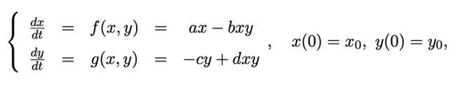
This ODE was originally designed for predator-prey relationship, but the principle applies equally for foraging animals. In fact, the population of forager and that of its prey are dependent on each other. If the quantity of food increases rapidly, it will allow a large number of foraging animals to survive. On the other hand, if the prey population becomes significantly small, there will not be enough food for foragers, which causes a decline in the number of foragers. Ultimately, the number of foragers and preys achieves an equilibrium. The following system of equations is based on the same principles:

1. The prey population, represented by x(t), increases when there is no encounter between forager and prey (+ax).
2. The foraging animal population, represented by y(t), diminishes when there is no encounter between forager and prey (-cy).
3. The number of interactions between two species is the product of their population density. This statement leads to the logical conclusion that the chance of an encounter is larger when the populations are larger. These encounters cause a decrease in prey population (-bxy) and an increase in the population of foraging animals (+dxy).

Conclusion

Ultimately, mathematical models are used to predict how animals behave when searching for food, as well as to describe the movement of foragers during patch selection. Although obtaining nutrients from food provides the animal with energy, searching for and capturing the food requires both time and energy. In order to maximize fitness, animals adopt a foraging strategy that provides the most benefit by maximizing the net energy gained. The Optimal Foraging Theory helps predict the best strategy used by an animal species to achieve this goal. Many mathematical models have been developed to explain various foraging behaviours and searching techniques of animals. In this essay, the applications of mathematical models have been examined through the examples of trail-laying Argentine ants and of honeybees in an environment containing two types of flowers. These models allowed us to represent the most general foraging patterns observed among different animals. However, it is important to keep in mind that the environment foragers live in is far more elaborated, which requires more complex mathematical models to describe foraging behaviours. Further adjustments of mathematical models should be continued, as it had been the case for the last decades.

References

Charnov, E. L. (1976). Optimal foraging, the marginal value theorem. Theoretical Population Biology, 9(2), 129-136. https://doi.org/https://doi.org/10.1016/0040-5809(76)90040-X

Ferreira, M. F. A. (2014). Stochastic Differential Equation Models in Population Dynamics [Master’s thesis, University of Coimbra]. marinaaferreira.files.wordpress.com.

LaScala-Gruenewald, D. E., Mehta, R. S., Liu, Y., & Denny, M. W. (2019). Sensory perception plays a larger role in foraging efficiency than heavy-tailed movement strategies [article]. Ecological Modelling, 404, 69-82. https://doi.org/10.1016/j.ecolmodel.2019.02.015

Leidus, I. (2016, July 24). File:Apis mellifera – Senecio paludosus – Keila.jpg. Wikimedia Commons. Retrieved November 25, 2021, from https://commons.wikimedia.org/wiki/File:Apis_mellifera_-_Senecio_paludosus_-_Keila.jpg

Lozano, G. A. (1998). Parasitic Stress and Self-Medication in Wild Animals. Advances in The Study of Behavior, 27, 291-317.

MacArthur, R. H., & Pianka, E. R. (1966). On Optimal Use of a Patchy Environment. The American Naturalist, 100(916), 603-609. http://www.jstor.org/stable/2459298

Ramsch, K., Reid, C., Beekman, M., & Middendorf, M. (2012). A mathematical model of foraging in a dynamic environment by trail-laying Argentine ants. Journal of Theoretical Biology, 306, 32-45. https://doi.org/10.1016/j.jtbi.2012.04.003

Reid, C., Latty, T., & Beekman, M. (2012). Making a trail: Informed Argentine ants lead colony to the best food by U-turning coupled with enhanced pheromone laying. Animal Behaviour, 84, 1579-1587. https://doi.org/10.1016/j.anbehav.2012.09.036

The Editors of Encyclopaedia Britannica. (2017, May 31). Brownian motion. Encyclopaedia Britannica. Retrieved November 25, 2021, from https://www.britannica.com/science/Brownian-motion

Viswanathan, G. M., Buldyrev, S. V., Havlin, S., da Luz, M. G., Raposo, E. P., & Stanley, H. E. (1999). Optimizing the success of random searches. Nature, 401(6756), 911-914. https://doi.org/10.1038/44831

Vittori, K., Talbot, G., Gautrais, J., Fourcassié, V., Araújo, A. F., & Theraulaz, G. (2006). Path efficiency of ant foraging trails in an artificial network. J Theor Biol, 239(4), 507-515. https://doi.org/10.1016/j.jtbi.2005.08.017

Waddington, K. D., & Holden, L. R. (1979). Optimal Foraging: On Flower Selection by Bees. The American Naturalist, 114(2), 179-196. https://doi.org/10.1086/283467