Mathematical Models of Predator-Prey Population Dynamics 

Andrew Xie, Dalya Messaoudi, Laurier Gauvin,  Reefah Kabir

Abstract

Biology and ecology are often viewed through a lens of pure chemistry or physics. However, these two fields do not serve particularly well when analyzing systems, namely ecosystems, at a macro level. Indeed, as we will discuss, it is mathematics, or alternatively biomathematics, that serves us in aggregating large amounts of data to then attempt to model the populations of species within an ecosystem. We will also highlight that whilst these models can be extremely insightful, they are fundamentally imperfect, from the often-limited resources available for data collection to the near infinite number of variables that tend to skew the true size of populations in one direction or another. We will discuss a few of these specific factors, specifically disease, contamination, and predator-induced breeding suppression, to demonstrate that we can nonetheless gain a slightly more sophisticated understanding of a given ecosystem once we isolate the known variables and limit the interplay between them. It is with these incremental advancements that we can eventually gain a more thorough understanding of the ecosystems we live in and interact in on a daily basis so that we can hopefully come to recognize and act on the consequences we have on them.

Introduction

It is no question that there is a significant relationship between the population size of predator and prey (Blasius et al., 2020) – the rate of increase of the number of prey species gets smaller as the number of predators increases, whereas the rate of increase of the number of predator species gets larger as the number of prey species increases (Volterra, 1926). When looking at the perspective of the predator, this relationship can be attributed to the Metabolic Theory of Ecology, which states the carrying capacity of a species is linearly dependent on the abundance of the limiting resource (Brown et al., 2004). For the prey, this can be seen through a simple exercise in numbers: as the number of predators goes up, the more prey is consumed, leading to a lower/negative growth rate in the population, and vice versa.

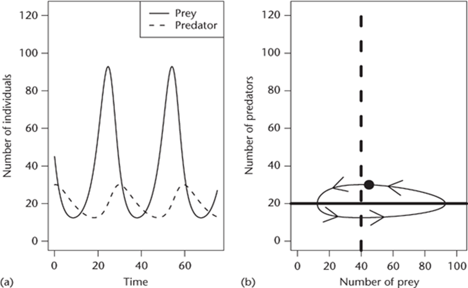
These principles gives rise to an oscillation in the populations of the prey and predator species – when treating the sizes of the populations as a function of time, the periods of oscillation are generally same between the two species, however, the predator species and prey species reaches a maximum and minimum population at different times, with the predator species distinctly lagging behind the prey species (Fig. 1) (Volterra, 1926).

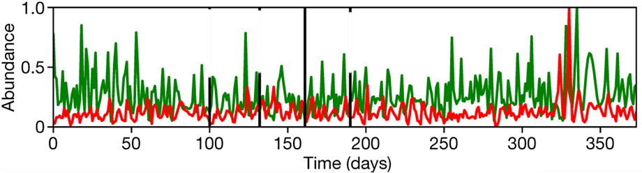
When we attempt to find a mathematical relationship between predator prey relationships, however, it is extremely challenging to not only compute an appropriate model, but also gather good data for the proper formulation of the models as well. Experiments that occur in a lab setting, although useful for gathering data, oftentimes provides results that are too idealized; certain interactions between the species being studied and their natural environment are challenging, if not possible, to simulate in laboratory conditions while simultaneously investigating predator-prey oscillations, such as disease, interactions from organisms outside the scope of the experiment, and the natural variance in environmental conditions (Kendall et al., 1999). On top of that, laboratory experiments have a great challenge in that they are very often unable to sustain the oscillations seen in nature for many generations, though new research has been able to prove that these systems are able to exist without further outside intervention (Blasius et al., 2020). Gathering data from nature is no better; the amount of environmental variance, the presence of competing mechanisms, and natural disturbances to the oscillation regime makes this data profusely challenging to use (Kendall et al., 1999; Liu & Chen, 2003).

This poses several questions: Can such a complex relationship be generalized through something as decisive as a mathematical model? Is it even practical to create and apply a mathematical model with all the different factors that must be considered? Are there any new understandings to be obtained with models that are not able to accurately provide a quantitative prediction?

When discussing questions like this, however, it is critical to remember the original intention of creating these mathematical models; as Kendall et al. (1999) states: “many of these models were originally designed to answer qualitative questions about population dynamics, and there is no way that they can encompass all the factors affecting a population.” The creation, application, and rejection of these models have led to some critical insights into our understanding of population dynamics in predator-prey relationships (Kendall et al., 1999). For example, models that account for adaptability of the species involved in the predator-prey relationship has a significant effect on the stability and pattern of population oscillation (Ives & Dobson, 1987; Mougi & Iwasa, 2010).

Furthermore, as models are further developed in their scope and degree of complexity, it is possible that a model that able to accurate quantitative predictions will eventually be reached, providing scientists with further understanding of the natural world and its internal clockwork.

The Lotka-Volterra Model

One of the most prominently used mathematical models for predator-prey relationships is the Lotka-Volterra model (Ayala et al., 1973). Derived by Lotka in 1925 and separately by Volterra in 1926, the model presents a logistic function to explain the oscillatory nature of populations in predator-prey systems (Berryman, 1992). The most elementary version of this model can be expressed through two equations:

{dx\over dt}=rx-αxy

{dy\over dt}=βxy-Dy

where dx/dt is the rate of change of the prey species, dy/dt is the rate of change of the predator species, x is the number of prey, y is the number of predators, r and D are constants that describe the rates of change in the populations in each respective organism independent of predator-prey interactions, and α and β describe the impact of predator-prey relationships on each species' numbers (Berryman, 1992; Wangersky, 1978).

The elementary model, however, runs into the issue that the prey population grows indefinitely in the absence of a predator species, which is practically impossible. To rectify this, a term of density-dependence is generally introduced into the equation modelling the prey population:

{dx\over dt}=rx(1-{x\over K})-axy

in which K is treated as the carrying capacity (Ayala et al., 1973; Berryman, 1992; Wangersky, 1978).

By solving equations that have their basis in the Lotka-Volterra model, it creates a series of inherently oscillatory ellipses that are dependent on the condition that the system started with (Fig. 2) (Berryman, 1992).

However, there are several significant variables that are unaccounted for with this model. As Ayala et al. (1973) points out “it does not take into account the age of organisms, their sex, nor genetic differences between them. It also ignores time lags and assumes that competitive interactions, both intra- and interspecific, are linear.” Because all these variables are unaccounted for, using experimental data to create a Lotka-Volterra model is likely to result in a quantitatively inaccurate model. Furthermore, with its roots in being a logistic function, the Lotka-Volterra model makes certain assumptions that have absolutely no biological justification, one of the most serious being that it requires cause and effect to coincide, something that practically does not occur in a natural predator-prey relationship (Ayala et al., 1973). Certain corrections can be made in order to account for some of these variables and assumptions, however, they increase the complexity of these models by several orders of magnitude (Ayala et al., 1973).

Why is the Lotka-Volterra model then used so widely over other models? Firstly, it stems from its practicality compared to everything else we have; as a logistic function, the model itself is easily manipulatable, it “fits many population growth experiments about as well as any biological data are ever fitted,” and it can be accurate for specific systems such as ones involving protazoans (Ayala et al., 1973). As well, many of the insights scientists have gathered in population dynamics has stemmed from variations and transformations of the basic Lotka-Volterra model into ones that are more precise, an example being the aforementioned introduction and development of the carrying capacity constant (Ayala et al., 1973; Berryman, 1992).

One of the most interesting applications of the Lotka-Volterra model to bioengineering is in disease-modelling. By modelling COVID-19 as a predator population and humans as the prey, scientists have been able to create an accurate model for transmission that can be used to simulate various public-policy shifts (Mohammed et al., 2021). However, when looking at disease dynamics in predator-prey populations, a more parameterized model may be more appropriate: the SIR (Susceptible-Infectious-Recovered) inspired predator-prey model.

Infectious Diseases and their Effects in Predator-Prey Population Dynamics

As previously mentioned, the Lotka-Volterra model is effective at analyzing the population dynamics between predators and prey. However, this relationship becomes more complex with the presence of infectious diseases. Indeed, either prey or predator can become vectors for viruses, parasites or bacteria enabling spread of diseases within and between species, but they can also become the solution to limiting the propagation of pathogens further affecting population sizes.

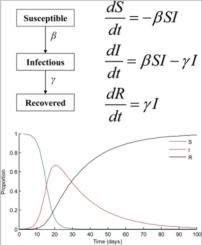
To study the impact of the infections on a certain species, the SIR (Susceptible-Infectious-Recovered) mathematical model can be used (Luz et al., 2010). The population is divided into three categories as suggested by the name of the model (Fig. 3). The susceptible group (S) consists of all organisms at risk of contracting the infectious disease, but who are not infected (Luz et al., 2010). The infectious group (I) includes the ones contracting the diseases with or without symptoms. The recovered group (R) consists of those who were able to heal from the infection, alive. This model is mainly composed of three ordinary differential equations accounting for the rates of change of the number of entities from each of the three categories over time as well as accounting for constant rates of transmission (β) and recovery (γ) (Luz et al., 2010). In the specific example provided by the graph of Figure 3, the initial number of infected organisms is 1, and over time, the numbers for group S decrease and the ones for group R increase with assumption of long-term immunity. The numbers for group I reach a maximum only to decline again.   

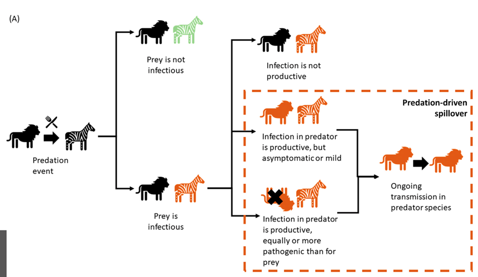
When it comes to predator-prey dynamics, there are a few ways infectious diseases can be transmitted or stopped and these further impact population changes. Within the same species, pathogens can be transmitted through direct contact or contamination due to the environment. This is case for the chronic wasting disease (CWD) in deer and elk (Nichols et al., 2015). As shown in the Figure 4, there can be multiple outcomes to predation with regards to disease transmission depending on the species and the pathogen (Malmberg et al., 2021). As one of the possible outcomes, although a predator may be exposed to the infected prey, it may not catch its disease. This can be due to the predator having an inadequate biological system which would stop the disease from impacting them but can still be released through feces (Nichols et al., 2015). Another explanation could be that, although the prey is being consumed, the predator's body has an ability to deactivate the pathogen. For example, the intestines of the predator contain enough enzymes to lyse and inactivate infected prey cells which prevents infection (Das, 2016). Another way an infection is deactivated is through the low pH of the stomach which can destroy pathogens and this is the case for vultures when consuming carcasses of animals that had tuberculosis (Malmberg et al., 2021). In fact, these processes have sparked a few studies that consider the role of harvesting to decrease infected prey populations, restrict the propagation of pathogens as predators have a tendency to hunt down prey that are more ill as well as limit prey and predator oscillations, especially in the cases of avian influenza and the flu (Das, 2016, 2020). Another outcome of predation would be the transmission of disease from prey to predator, ranging from mild to worse symptoms once infected (Fig. 4) (Malmberg et al., 2021). For instance, the canine distemper virus originating from domestic dogs was found in Serengeti lions causing fatal disease with signs of pneumonia and encephalitis (Roelke-Parker et al., 1996).

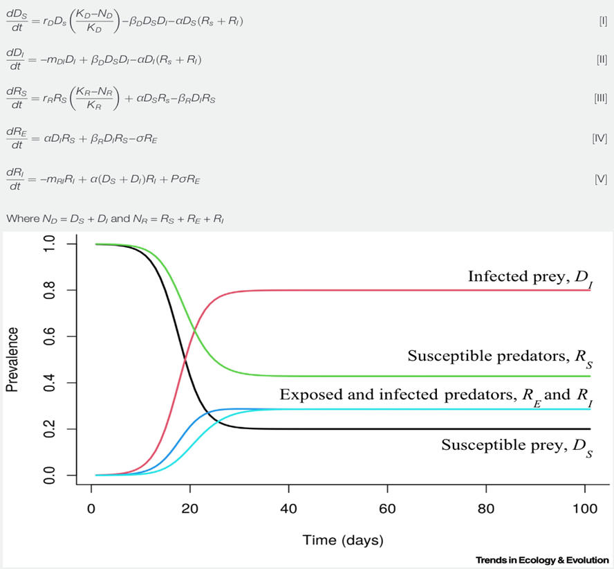
One of the many suggested mathematical models denoting the populations of predators and preys subject to infectious diseases considers predation as well as direct contact as ways of transmission which affect both predators (R) and prey (D) (Fig. 5). As simplifications, this model doesn't account for the recovery group and assumes that organisms once infected will stay in the infected group. It also adds an exposed group (R_E) for organisms coming in contact to a disease but that are not instantly infected alongside the infected (D_I and R_I) and susceptible groups (D_S and R_S). The model also adds parameters such as carrying capacities (K_D and K_R), growth rates specific to species while assuming logistic growth (r_D and r_R), rates of consumption of prey (α), disease-specific death rates (m_DI and m_RI), transmission rates from prey to other prey (β_D ) and from prey to predator (β_R ), rates for the transition from the exposed to the infectious group (σ) as well as the fraction of infected predators that can spread the pathogens (P) (Fig. 5). It is important to consider that this model, like other mathematical models, is a simplification of the cause and effects of infections in predator-prey relationships since it doesn't encompass recovery rates, predators being a limiting factor of disease spread for certain diseases as well as scenarios of predators being the source of infections.

This model, derived from the Lotka-Volterra model,  includes five ordinary differential equations indicating the rates of change of the number of infected prey (dD_s/dt), susceptible prey (dD_I/dt), exposed predators (dR_E/dt), susceptible predators (dR_S/dt) and infected predators (dR_I/dt) (Fig.5) (Malmberg et al., 2021). For initial conditions where there are 1/1000 infected prey, 10 susceptible predators and 0 infected or exposed predators, the number of infected prey (D_I) increases more than that of infected predators (R_I). The susceptible prey group (D_s) experiences a steeper decline than the susceptible predator group. Finally, groups reach an equilibrium state over time.

Studying the effects of infections on the populations of predators and prey is also effective when looking at the zoonotic diseases that affect human populations. By creating mathematical disease models for animals, we can evaluate the risks humans have to be infected by animal-driven diseases and thus, take preventive measures such as vaccinations to avoid epidemics. 

Contaminants and their Effects in Predator-Prey Population Dynamics

Whilst the general mathematical models of the population dynamics of a given ecosystem can generally be calculated with enough time, manpower, and computational ability, measuring the precise contribution of each particular factor influencing this dynamic is a much more difficult task. Nevertheless, it remains just as much, if not more, important. One such example of these factors is the presence, or lack thereof, of contaminants and/or chemicals in a given environment. One could assume that a substance that is of similar toxicity for all animals in a given environment would have similarly harmful effect on all species, and whilst that may be true in some instances (Ross et al., 2021), we will discuss the higher order effects of introducing harmful foreign substances into an environment which invariably affect some species more than others.

One particularly topical instance of such contamination is the increasing problem of microplastics in nearly all natural habitats around the world. The problem is in fact so ubiquitous that the concentration of microplastics in the North Pole is nearly identical to that in the Hudson Bay (Huang et al., 2020). Due to this increasing problem, many studies have come out in recent years trying to model the precise effects that this factor would have on predator-prey populations. A recent paper by Huang et al. (Ross et al., 2021) attempted to model this exact thing and found that whilst predators and prey populations did not suffer the same consequences as a result of adverse reactions to microplastics, the concentration of microplastics changed the degree to which each individual group suffered. The overall trend nonetheless was found to be that predators invariably suffered worse outcomes than prey, lining up with broader research on the study of biomagnification. At lower levels of microplastics both predators and prey numbers fluctuate somewhat, however it is to a minimal and more or less equal degree. As microplastic concentration progressively increases, more predators and prey begin to die as a result of the contaminant, but prey populations nonetheless increase as a result of the decrease in predation. Of course, this does not mean that microplastics necessarily have a positive evolutionary impact on the prey, as even when their natural predators go extinct, high concentrations of microplastics eventually tend to bring the population of prey down to zero.

If these theoretical findings are proven to hold through more applied research, measuring the fluctuation in the ratio of predators to prey in an ecosystem could potentially be a tool used to better diagnose the precise ecological balance of an ecosystem known to be particularly contaminated, by microplastics or otherwise. Whilst most predator and prey populations do fluctuate to a certain extent, sometimes greatly (Jansen, 2001), with accurate and up to date data, a seemingly positive sign such as an increase in prey population could be indicative of impending ecological collapse, potentially leaving to a large enough buffer period to respond accordingly.

In this previous example, the general assumption was that each species had a similar sensitivity the contaminant, in that case microplastics, but that is in fact not always the case. Indeed, even more general models on the spread of contaminants tend to reach their limitations when individual species demonstrate varying sensitivities to a particular foreign substance (Huang et al., 2015). Despite the phenomenon of biomagnification, prey that are particularly susceptible to the negative effects of a contaminant could find themselves to be the sole species in a habitat that would come to go extinct. This would be because part of the population would be dying as a result of the particular toxin, but it could also be caused an increase in general ailments and disorders, rendering the species more vulnerable to predation. This increase in vulnerability would in turn lead to increased predation until the species of prey is no more.

Whilst it is surprising the extent to which we can model the predator-prey dynamics of a given ecosystem, it remains particularly important to push the field forward, particularly in regards to contaminants in ecosystems, as with increased human development and urbanization, it will become more and more important to measure and therefore prevent the many adverse effects that we can have on the many diverse ecosystems in the world.

Predator-Induced Breeding Suppression and their Effects in Predator-Prey Populations Dynamics

Another phenomenon which has been shown to have a potential effect on predator-prey population dynamics are anti-predator responses. One of these responses which is currently being researched is predator-induced breeding suppression (PIBS) (Jochym & Halle, 2012; Ruxton & Lima, 1997). It has been observed that during a strong predation, the pressure produced causes small mammals to suppress breeding (Jochym & Halle, 2012; Roy et al., 2020; Ruxton & Lima, 1997).  Being a non-breeding individual comes with advantages such as being capable of avoiding predation as opposed to an individual in a reproductive state (Ruxton & Lima, 1997). In a study conducted by Graeme Ruxton and Steven Lima (1997), a model was developed to investigate the effect of predator-induced breeding suppression (PIBS) on predator-prey dynamics. The model divides the prey population into two subpopulations. Breeding population (B) and breeding suppressing population (S). The breeding population as opposed to the breeding suppressing population is exposed to the predator population (P). 

This model uses rate theory to study the predator-prey dynamics. The rate of change in the predator population is defined as follows:

{dP\over dt}={(ε I_m  B P)\over (B+B_0 )} - μP  (1)

where e represents a constant of efficacy for prey converting to predators, I_m is the maximum intake rate, which can also be defined as the inverse of prey handling time, and m is the constant per capita death rate.

The rate of change of individuals moving from the breeding population into the suppressing population is:

∅(P,B)={(P∅_m)\over (P+ P_0+aB)} (2)

where ∅_m is the maximum rate, a is the parameter controlling the per capita rate of movement out of the breeding population. The rate of change in the suppressing population is:

{dS\over dt}= ∅(P,B)B- αS  (3)

where a is the parameter describing the per capita rate of movement from the suppressing population to the breeding population.  Finally, the fecundity of the breeding population is also taken into consideration in this model and is described by a simple logistic

{dB\over dt}=rB(1-{B\over K})- {I_m B P\over (B+B_0}-∅(P,B) B+αS (4)

The variable r represents the maximum population growth rate whereas K is the carrying capacity (Ruxton & Lima, 1997).

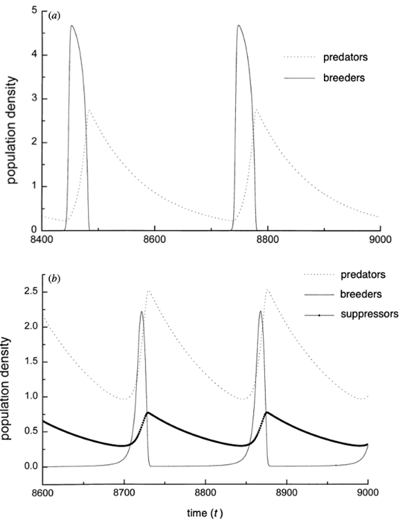
The authors of the paper used the steady states of the different equations in the model to determine the variations in the predator and prey populations (Ruxton & Lima, 1997). By varying fm (maximum rate of change of individuals moving from the breeding population into the suppressing population) positively and significantly i.e., by increasing the breeding suppression, the predator population size has been observed to be unaffected. However, the prey population increases. This effect contributes into stabilizing the predator-prey cycle if the suppression is significantly strong. This happens because the frequency of existing oscillations increases (Ruxton & Lima, 1997). Figure 6 showcases the two of the three possible scenarios with breeding suppression. In Figure 6a, f_m  à 0. Consequently, φ (P, B) also goes to zero. This means there is no movement of individuals from the breeding to the suppressor population. We can determine from the same figure that the abrupt growth of the predator population causes the prey population to crash. However, the change is adjusted following a decline in the predator population and recreated once the predator population grows again. This cycle keeps going as long as both populations of predator and prey exist and whether there is suppression or not (Roy et al., 2020; Ruxton & Lima, 1997).  In Figure 6b, where breeding suppression is present but not significant, we can see that a third curve comes into play: the suppressing population. Because of the presence of the suppressing population (considered invulnerable for predation), the breeding one recovers faster from a population drop (Jochym & Halle, 2012; Ruxton & Lima, 1997). This happens because individuals from the suppressing population return into a breeding state. This behaviour allows conservation of the prey population and allows for stability of predator-prey cycle. The last scenario where there is a strong breeding suppression will allow for total stability of the cycle (Ruxton & Lima, 1997).

Conclusion

In conclusion, predator-prey dynamics aren't straight forward – they do not merely encompass the chase and consumption of prey and cannot always be accurately represented by the Lotka-Volterra model, although it is a useful model for many studies for its simplicity. In fact, many factors such as toxic components including microplastics from the environment, the presence of infectious diseases in species as well as anti-predator behaviours including breeding suppression may require a few modifications of the simplistic Lotka-Volterra model giving rise to different and more complex mathematical models describing the multifaceted interspecies relationships. As such, predator-prey mathematical models can be used for bioengineering applications, such as disease modelling for COVID-19 and toxicity modelling for contaminated ecosystems.

References:

Ayala, F. J., Gilpin, M. E., & Ehrenfeld, J. G. (1973). Competition between species: Theoretical models and experimental tests. Theoretical Population Biology, 4(3), 331-356. https://doi.org/https://doi.org/10.1016/0040-5809(73)90014-2

Berryman, A. A. (1992). The Orgins and Evolution of Predator-Prey Theory. Ecology, 73(5), 1530-1535. https://doi.org/https://doi.org/10.2307/1940005

Blasius, B., Rudolf, L., Weithoff, G., Gaedke, U., & Fussmann, G. F. (2020). Long-term cyclic persistence in an experimental predator–prey system. Nature, 577(7789), 226-230. https://doi.org/10.1038/s41586-019-1857-0

Brown, J. H., Gillooly, J. F., Allen, A. P., Savage, V. M., & West, G. B. (2004). Toward a metabolic theory of ecology. Ecology, 85(7), 1771-1789. https://doi.org/https://doi.org/10.1890/03-9000

Das, K. p. (2016). A study of harvesting in a predator–prey model with disease in both populations. Mathematical Methods in the Applied Sciences, 39(11), 2853-2870. https://doi.org/https://doi.org/10.1002/mma.3735

Das, K. P. (2020). Proper Predation and Disease Transmission in Predator Population Stabilize Predator–Prey Oscillations. Differential Equations and Dynamical Systems, 28(2), 295-313. https://doi.org/10.1007/s12591-016-0324-8

Hartvigsen, G. (2012). Predation (Including Parasites and Disease) and Herbivory. In eLS. John Wiley & Sons, Ltd. https://doi.org/https://doi.org/10.1002/9780470015902.a0003310.pub2

Huang, Q., Lin, Y., Zhong, Q., Ma, F., & Zhang, Y. (2020). The Impact of Microplastic Particles on Population Dynamics of Predator and Prey: Implication of the Lotka-Volterra Model. Scientific Reports, 10(1), 4500. https://doi.org/10.1038/s41598-020-61414-3

Huang, Q., Wang, H., & Lewis, M. A. (2015). The impact of environmental toxins on predator–prey dynamics. Journal of Theoretical Biology, 378, 12-30. https://doi.org/https://doi.org/10.1016/j.jtbi.2015.04.019

Ives, A. R., & Dobson, A. P. (1987). Antipredator Behavior and the Population Dynamics of Simple Predator-Prey Systems. The American Naturalist, 130(3), 431-447. https://doi.org/10.1086/284719

Jansen, V. A. A. (2001). The Dynamics of Two Diffusively Coupled Predator–Prey Populations. Theoretical Population Biology, 59(2), 119-131. https://doi.org/https://doi.org/10.1006/tpbi.2000.1506

Jochym, M., & Halle, S. (2012). To breed, or not to breed? Predation risk induces breeding suppression in common voles. Oecologia, 170(4), 943-953. https://doi.org/10.1007/s00442-012-2372-2

Kendall, B. E., Briggs, C. J., Murdoch, W. W., Turchin, P., Ellner, S. P., McCauley, E., Nisbet, R. M., & Wood, S. N. (1999). Why Do Populations Cycle? A Synthesis of Statistical and Mechanistic Modeling Approaches. Ecology, 80(6), 1789-1805. https://doi.org/https://doi.org/10.1890/0012-9658(1999)080[1789:WDPCAS]2.0.CO;2

Liu, X., & Chen, L. (2003). Complex dynamics of Holling type II Lotka–Volterra predator–prey system with impulsive perturbations on the predator. Chaos, Solitons & Fractals, 16(2), 311-320. https://doi.org/https://doi.org/10.1016/S0960-0779(02)00408-3

Luz, P. M., Struchiner, C. J., & Galvani, A. P. (2010). Modeling Transmission Dynamics and Control of Vector-Borne Neglected Tropical Diseases. PLOS Neglected Tropical Diseases, 4(10), e761. https://doi.org/10.1371/journal.pntd.0000761

Malmberg, J. L., White, L. A., & VandeWoude, S. (2021). Bioaccumulation of Pathogen Exposure in Top Predators. Trends in Ecology & Evolution, 36(5), 411-420. https://doi.org/10.1016/j.tree.2021.01.008

Mohammed, W. W., Aly, E. S., Matouk, A. E., Albosaily, S., & Elabbasy, E. M. (2021). An analytical study of the dynamic behavior of Lotka-Volterra based models of COVID-19. Results in Physics, 26, 104432. https://doi.org/https://doi.org/10.1016/j.rinp.2021.104432

Mougi, A., & Iwasa, Y. (2010). Evolution towards oscillation or stability in a predator–prey system. Proceedings of the Royal Society B: Biological Sciences, 277(1697), 3163-3171. https://doi.org/doi:10.1098/rspb.2010.0691

Nichols, T. A., Fischer, J. W., Spraker, T. R., Kong, Q., & VerCauteren, K. C. (2015). CWD prions remain infectious after passage through the digestive system of coyotes (Canis latrans). Prion, 9(5), 367-375. https://doi.org/10.1080/19336896.2015.1086061

Roelke-Parker, M. E., Munson, L., Packer, C., Kock, R., Cleaveland, S., Carpenter, M., O'Brien, S. J., Pospischil, A., Hofmann-Lehmann, R., Lutz, H., Mwamengele, G. L. M., Mgasa, M. N., Machange, G. A., Summers, B. A., & Appel, M. J. G. (1996). A canine distemper virus epidemic in Serengeti lions (Panthera leo). Nature, 379(6564), 441-445. https://doi.org/10.1038/379441a0

Ross, P. S., Chastain, S., Vassilenko, E., Etemadifar, A., Zimmermann, S., Quesnel, S.-A., Eert, J., Solomon, E., Patankar, S., Posacka, A. M., & Williams, B. (2021). Pervasive distribution of polyester fibres in the Arctic Ocean is driven by Atlantic inputs. Nature Communications, 12(1), 106. https://doi.org/10.1038/s41467-020-20347-1

Roy, J., Barman, D., & Alam, S. (2020). Role of fear in a predator-prey system with ratio-dependent functional response in deterministic and stochastic environment. Biosystems, 197, 104176. https://doi.org/https://doi.org/10.1016/j.biosystems.2020.104176

Ruxton, G. D., & Lima, S. L. (1997). Predator-induced breeding suppression and its consequences for predator-prey population dynamics. Proceedings of the Royal Society of London. Series B: Biological Sciences, 264(1380), 409-415. https://doi.org/doi:10.1098/rspb.1997.0058

Volterra, V. (1926). Fluctuations in the Abundance of a Species considered Mathematically1. Nature, 118(2972), 558-560. https://doi.org/10.1038/118558a0

Wangersky, P. J. (1978). Lotka-Volterra Population Models. Annual review of ecology and systematics, 9, 189-218. http://www.jstor.org/stable/2096748