Deciphering Daphnia Dynamics: A Mathematical Odyssey into Aquatic Ecosystems

Eva Otell, Iris Sun, Marwan Sobh, Xinying Wang, Rémi Ouellette

Abstract

Amongst all the chaos found in aquatic ecosystems, Daphnia emerges as a small yet pivotal player, embodying the complexity and adaptability of life. This study presents a mathematical journey into Daphnia populations, revealing the sophisticated interplay between their unique reproductive strategies, survival tactics, and trophic interactions. Cyclical parthenogenesis, a fascinating reproductive phenomenon where Daphnia alternates between asexual and sexual reproduction in tune with environmental cues, is explored. Game theory is used to investigate this adaptive strategy, shedding light on its evolutionary importance in fluctuating habitats. Their trophic relationships, particularly during algal blooms and encounters with predators like Chaoborus are also closely observed. Daphnia demonstrates remarkable behavioral adaptations, ranging from morphological defensive strategies against predators to the strategic delay of reproduction as a calculated survival gamble. These adaptations are illustrated through various mathematical models. Daphnia‘s enigmatic swimming behavior is also uncovered through their horizontal migrations, their slowdown in swimming speed under predator-induced stress, and their diel vertical migrations, a daily rhythmic movement influenced by light and predation. This paper not only unravels the mathematical tapestry of Daphnia populations but also highlights their crucial role in maintaining ecological balance within the aquatic ecosystems.

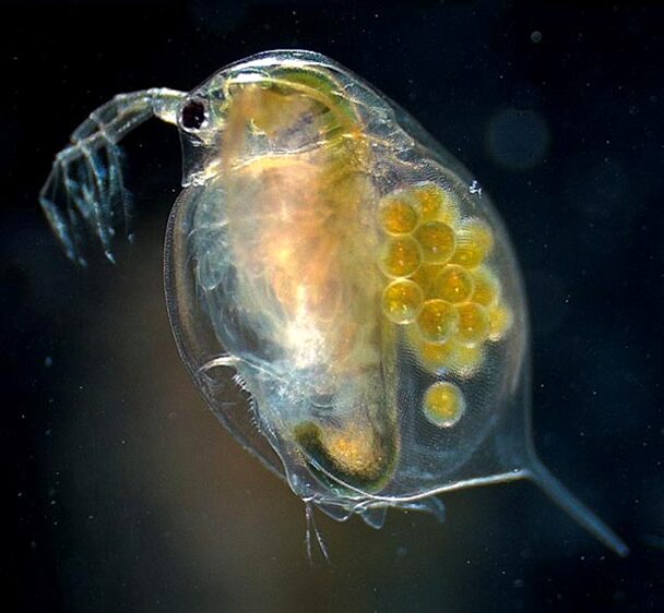
Fig. 1. Daphnia magna (Adult Female) (Stoeckel & Siriwardena, 2022).

Introduction

Daphnia, freshwater crustaceans commonly known as water fleas, play a significant role in the food web and respond dynamically to environmental cues and predator interactions. Understanding their adaptations, behaviours, and population dynamics provides valuable insights into freshwater ecosystems. A key focus is Daphnia‘s response to predation risk. Examining morphological changes and altered swimming behaviours reveals the adaptive strategies employed by Daphnia to survive in the presence of threats. Additionally, the impact of predator-induced cues on reproductive and migratory patterns adds complexity to their ecological role. This paper also explores the interaction between Daphnia and algae, highlighting the crucial role of nutritional dynamics in Daphnia-algae systems. Factors such as food availability and predation pressure contribute to the intricate ecological relationships within freshwater ecosystems. This paper unveils how water fleas’ survival and reproductive success are finely tuned by factors ranging from protective adaptations to complex predator-prey dynamics. Through a multifaceted examination incorporating game theoretic frameworks, quantitative modelling techniques, and empirical commentaries, it is possible to advance comprehension of ecological dynamics and illuminate the indispensable functions performed by this Cladoceran.

Population dynamics

Overview of D. magna’s population dynamics

Cyclic parthenogenesis greatly affects the population dynamics of D. magna. Key studies reveal the species’ adaptability through amictic parthenogenesis in challenging conditions. The link between offspring size, maternal age, and ecological costs provides insights into population fitness optimization. The population dynamics of D. magna led to structured population models, such as the Sinko-Streifer model, unveiling complexities in modelling D. magna‘s dynamics. This concise insight aims to illuminate the species’ unique reproductive strategies and population dynamics, enhancing the understanding of its adaptability in diverse environments.

Cyclical parthenogenesis in D. magna

Daphnia magna employs cyclical parthenogenesis as its primary reproductive strategy, giving rise to both male and female descendants solely through parthenogenesis in response to environmental cues, such as food availability and population density. This approach supports rapid population growth under favourable conditions and the development of resilient resting eggs capable of withstanding harsh environments (Goitom et al., 2018). The significance of cyclical parthenogenesis becomes apparent in its profound impact on population dynamics, fostering swift expansion during favourable conditions and resulting in elevated population densities. Additionally, the production of resting eggs ensures the species’ endurance in unfavourable conditions, securing survival and eventual re-establishment when environmental circumstances improve. This cyclical pattern shapes D. magna‘s overall population dynamics, contributing to its persistence across diverse environments (Goitom et al., 2018).

Moreover, the distinctive nature of cyclical parthenogenesis in D. magna reduces genetic diversity, as most individuals become replicas of the pioneering founders. When faced with adverse conditions, the species switches to amictic parthenogenesis, producing genetically identical offspring and facilitating the rapid expansion of clonal lineages (Decaestecker et al., 2009). While this strategy may temporarily diminish genetic diversity, it accelerates population increases, as mentioned earlier, and facilitates colonization of new habitats by encouraging swift growth. The reproductive cycle, depicted in Figure 2 (Decaestecker et al., 2009), outlines stages such as sexual reproduction, ephippial egg production, and amictic parthenogenesis, offering a visual representation for comprehending D. magna‘s reproductive strategy and its effects on population dynamics. In summary, the species’ ability to switch between sexual and asexual reproduction in response to environmental conditions and the production of resting and ephippial eggs contributes to its resilience and distinct population growth patterns in diverse environments.

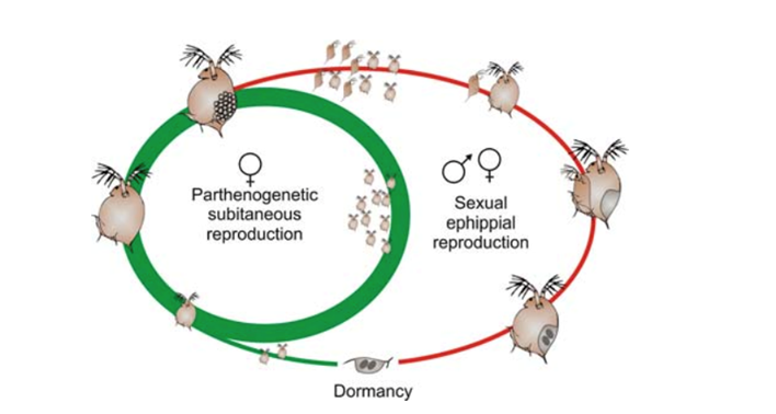
Fig. 2. The cyclically parthenogenetic life cycle of Daphnia. Parthenogenetic reproduction occurs for one to several generations under favourable circumstances (green). Long-lived dormant eggs are produced by sexual reproduction (red), and these eggs can hatch when favourable environmental circumstances are once again met. Some taxa create asexually dormant eggs by excluding the male from the cycle (Decaestecker et al., 2009).

Offspring size and population dynamics

The relationship between offspring size and population dynamics in D. magna, a key area of research with implications for the species’ reproductive success and overall population growth, has been extensively studied by scientists seeking to better understand how these interconnected factors impact the long-term sustainability of this species. Several investigations into this relationship have yielded useful understandings into the aspects that decide descendant magnitude and its consequences for the changing nature of numbers over time.

Boersma (Boersma, 1997) conducted a study to investigate the relationship between the age of the mother and the size of her offspring in D. magna. The study aimed to assess at what age of the mother the optimal offspring size was produced. The optimal offspring size was defined as the size of the offspring yielding the highest parental fitness, which translates to the highest juvenile fitness per unit effort put into these juveniles. The study found that the youngest females produced offspring with the highest juvenile fitness per unit effort and hence concluded that offspring produced by these females were of optimal size. Larger offspring produced by older females were estimated to yield only 70 % of the potential fitness of optimally sized offspring (Boersma, 1997).

Another study by Tagg (Tagg, 2004) explored the ecological cost of sexual reproduction in cyclically parthenogenetic Daphnia pulex, a close relative of D. magna. The study measured competition coefficients of genetically diverse and genetically uniform D. pulex populations to test a model of the ecological cost of mating. The study’s findings offer a glimpse into how cyclically parthenogenetic species like D. magna may numerically fluctuate over time, granting perspective on ecological and evolutionary impacts of sex in such tiny creatures (Tagg, 2004).

In addition, a study by (Einum et al., 2022) investigated the evolution of Daphnia population dynamics following invasion by a non-native predator. The study observed that predators are frequently observed to cause evolutionary responses in prey phenotypes, which can, in turn, influence population dynamics. In Figure 3, the analysis of population size trends in terms of both the number of individuals and total dry mass provides insights into the impact of the predator invasion on the Daphnia populations. The use of clones from before and after the invasion allows for a comparison of the population dynamics before and after the ecological disturbance, shedding light on the potential effects of the predator invasion on the Daphnia populations. Indeed, both the number of individuals and the totally dry mass of the organism increase post-invasion. The study’s findings highlight the complex interactions between predators and prey and their impact on population dynamics in Daphnia and other aquatic organisms (Einum et al., 2022).

These studies contribute to our understanding of the factors that influence offspring size, parental fitness, and population growth in D. magna (Boersma, 1997).

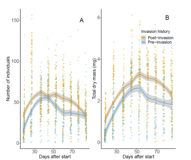
Fig. 3. Population size trends in terms of (A) number of individuals and (B) total dry mass for experimental populations of Daphnia originating from Lake Kegonsa (Einum et al., 2022).

Modeling population dynamics

In the simplest of cases of population dynamic modeling, the number of individuals can be very well estimated using a formula which considers the number of deaths, births, immigrating individuals and emigrating individuals in a given population. Using these factors, an initial equation can be written.

$\frac{dN}{dt} = rN$

Where N is the number of individuals at a time t

Equation 1: Simple ordinary differential equation to model population

In this equation, r is defined as the proportionality rate at which the population increases and is found using the factors mentioned above such as number of births. This equation makes sense as a method of representing population growth as the rate of increase of the number of individuals is proportional to the number of individuals at a given time. Solving this differential equation gives this formula.

$N = Ke^{rt}$

Where K is the initial number of individuals studied

Equation 2: General solution of equation 1

As it is possible to notice, there is a slight problem with this equation if it is to be used for real life situations, as the number of individuals would simply grow to infinity as time passes for any situation in which r is positive (Exponential & logistic growth). A solution to this would be using the logistic function as it allows us to place a limit on the number of individuals in a certain area. This limit would typically be determined according to certain factors such as the size of the zone in which the population lives. While this makes the model more realistic, there are other problems that must be addressed. The fact that Daphnia undergoes cyclical parthenogenesis makes it more complicated to model, as sexual and asexual reproduction must be considered in the same equation. The fact that Daphnia’s reproduction depends on the availability of food in their environment is also a factor that needs to be considered when creating such a model (Smith, 1963). These factors may be addressed with structured population models (SPMs), which “track the density of a population of individuals over time with respect to a physiologically structured variable, such as age or size” (Smith, 1963). SPMs are effective because they allow a precise way to put into equation the factors on which population growth is dependent, such as food abundance. One example of continuous structured population models would be the Sinko-Streifer model.

$\frac{\partial \eta(t,a,m)}{\partial t} + \frac{\partial \eta(t,a,m)}{\partial a} + \frac{\partial}{\partial m} \left[g(t,a,m)\eta(t,a,m)\right] = -D(t,a,m)\eta(t,a,m)$

Equation 3: Sinko-Strifer’s equation for a population density function depending on the age and mass variables (Sinko & Streifer, 1967).

The equation presented above results from the accumulation of different factors which are in play when observing the reproduction of a species. In this equation, the terms on the left are partial derivatives of the function η, which is the density of the population at a time t with individuals at an age a and at a mass m. Typically, when adding the partial derivatives with respect to each variable in a multiple variable function, the result is the derivative of the function itself, which isn’t the case here because of the insertion of the function g. The function g is the average growth rate of the animal studied at an age a, often analyzed experimentally. The D function is the death rate of the animals according to the same variables. Using this formula is quite complex and will not be explored in this paper (Sinko & Streifer, 1967). Researchers attempted to model population growth with inspiration from the Sinko-Streifer model and the result is the equation:

$\frac{\partial u(t,a)}{\partial t} + \frac{\partial u(t,a)}{\partial a} = -\mu_{\text{ind}}(a) \mu_{\text{dep}}(a,M(t))u(t,a)$

Equation 4: Model used for analyzing the population growth in D. magna (Smith, 1963).

In this experiment, the researchers used only two variables: time (t) and the age (a). The function for the density of the population is given by u and the mortality rate is given by μ, which is separated in two parts; μ_indwhich is independent on the density of the population, probably made up of natural deaths, and μ_dep which depends on the density rate, probably made up of casualties caused by lack of food or overcrowding. The function M represents the biomass at a time which makes sense since it is a variable for the density dependent mortality rate. The biomass depends on the number of individuals and the length of each one, which is set to follow some sort of logistic function. With some experimentation, these functions were able to be determined, but exploring them would need a paper on its own. The conditions in which the results are measured however, would change the function, which is why models can be found for different situations, such as when in presence of pesticides (Palamara et al., 2022) and predators (Palamara et al., 2022). In sum, there are plenty of models that can be made depending on how precise estimations have to be and depending on the factors that researchers want to study. Finding a model that takes into consideration all these factors and being 100 % accurate is near impossible, as nature often acts unpredictably, and maths simply won’t suffice.

Game theory

Natural selection operates in a frequency-dependent manner, meaning the fitness of a phenotype depends on its frequency relative to other phenotypes in the population (McNamara & Leimar, 2020). Biological game theory is therefore used to model such situations. The theory is concerned with the observable characteristics of organisms including behavior, morphological and physiological attributes (McNamara & Leimar, 2020). The two central methodological tools in biological game theory are the concepts of Nash equilibrium (Nash, 1950) and Evolutionarily Stable (Maynard Smith, 1972) (Huttegger & Zollman, 2013). Game theory in biology is built on several key concepts including actions, states, and strategies. Actions are defined in the widest sense, including behaviour, growth, and the allocation of the sex of offspring (McNamara & Leimar, 2020). State variables, on the other hand, are a description of some aspects of the current circumstance of an organism such as energy reserves, size, opponent’s last move, role, environmental temperature, social status and so on (McNamara & Leimar, 2020). These two concepts form strategies, which are genetically determined rules that specify the action taken as a function of the state of the organism (McNamara & Leimar, 2020). Strategies outline the actions to be taken under different circumstances. Hence, an organism adhering to a specific strategy might or might not perform a certain action, based on the situation it encounters (McNamara & Leimar, 2020). Moreover, the reproductive success of an individual is often tied to the strategy they use. This variation in reproductive success among different strategies influences the frequency of alleles in the population at genetic locations responsible for the range of possible strategies (McNamara & Leimar, 2020). Payoffs in biological games are in terms of fitness, a measure of reproductive success. In many cases the fitness of an individual can be described as the expected number of offspring in multiple generations (Hammerstein & Selten, 1994). The significance of the fitness concept lies in its ability to connect short run reproductive success with long run equilibrium properties (Hammerstein & Selten, 1994).

A large part of biological game theory focuses on the endpoints of evolutionary change where there is a formation of a stable strategy rather than evolutionary dynamics (McNamara & Leimar, 2020). Nash equilibrium is a key condition in this stability. It states that no player could improve their situation by unilaterally switching strategies (Huttegger & Zollman, 2013). In biology, this concept translates to evolutionary scenarios where organisms cannot gain any additional fitness by altering their behavior unless others do so as well. Nash equilibrium has two types. A population is said to be at a ‘pure strategy Nash equilibrium’ when it is monomorphic—all individuals adopt the same strategy which cannot be bettered by any mutant strategy (Huttegger & Zollman, 2013). Nash equilibrium also includes ‘mixed strategy equilibria’, which can be interpreted in two ways: as a single organism varying its strategy randomly or as a polymorphic population with multiple strategies coexisting (Huttegger & Zollman, 2013).

The concept of an Evolutionarily Stable Strategy (ESS) is intimately connected to Nash equilibria. An ESS is a specific type of pure strategy Nash equilibrium applied to evolutionary processes. The relation between Nash equilibrium and ESS is that while Nash equilibrium provides a static condition for stability, ESS adds an evolutionary dynamic. It describes a strategy that is not only a Nash equilibrium but also cannot be invaded by any alternative strategy that is initially rare (Hammerstein & Selten, 1994). This dynamic stability means that a monomorphic population using an ESS will remain monomorphic because no mutant strategy can invade and establish itself (Hammerstein & Selten, 1994). When considering the polymorphic interpretation, an ESS requires not only stability against the invasion of mutants but also against small perturbations of the relative frequencies already present in the population (Hammerstein & Selten, 1994).

A strategy (phenotype) s^* is an ESS if and only if the following two conditions are met:

$u(s^{*}, s^{*}) \geq u(s, s^*) \text{ for all alternative strategies }$ and

If $u(s^*, s^*) = u(s, s^*)$ , then $u(s^*, s)$ > $u(s, s)$ .

Equation 5: $u(x,y)$ represents the fitness (payoff) of a strategy x against y. The first condition states that s^* is in Nash equilibrium with itself (there is no other strategy earning a higher payoff against s^*). The second condition guarantees stability in case of a mutant strategy, s, that earns the same payoff against s^* by requiring that s^* is doing better against s than the mutant strategy against itself. The strategy s^*can be either a pure strategy or a mixed strategy (Huttegger & Zollman, 2013).

Daphnia populations may be monomorphic or polymorphic, depending on the environmental conditions. Under stable and favorable environments, all Daphnia individuals employ the same reproductive strategy (asexual reproduction) because it is the most efficient way to increase population size quickly (Ebert, 2022). When the environmental conditions deteriorate and lower the survival likelihood of asexual offspring, Daphnia population becomes polymorphic with the introduction of sexual reproduction, which brings genetic variability (Ebert, 2022). At the same time, Daphnia is able to detect kairomones. Consequently, they can change their body shape (e.g., develop helmets, neck–teeth, elongated tail spines), alter their life-history (e.g., size and age at maturity, offspring size), change behavior (phototaxis, swimming parameters). Moreover, Daphnia produces fewer and larger offspring when food is scarce and produces specific haemoglobin variants tailored to the partial oxygen pressure of the water. This adaptive phenotypic plasticity helps Daphnia to maintain a viable population in the face of changing environmental conditions and threats (Ebert, 2022).

These adaptations are the strategies Daphnia employs to resist the change in the environment. To determine if these changes are examples of ESS, the two conditions mentioned above need to be taken into consideration. For the switching between two reproductive strategies, in stable and favorable environments, asexual reproduction (strategy s^*) is employed by Daphnia because it allows adult females to produce clones (both females and males) of themselves without mating and thus contributing to a rapid population growth (La et al., 2014). Consequently, the fitness payoff of this strategy against itself is high and no alternative strategy is better in these conditions, satisfying the first condition for ESS. When the environment becomes less favorable, sexual reproduction is introduced (strategy s) (La et al., 2014). When the environment deteriorates, a new strategy (sexual reproduction) is introduced. Initially, it has equal fitness against s^* because it allows survival through genetic variability but doesn’t immediately increase the population size. However, if the strategy s^* (asexual reproduction) and s (sexual reproduction) yield the same payoff, the environmental shift makes s^* potentially advantageous for long-term survival due to genetic diversity, satisfying the second condition. Hence the switching between sexual and asexual reproduction can be considered as an ESS. It increases the probability that some offspring will possess traits that make them more suited to survive in challenging environments and acts as a buffer against threats like disease, environmental shifts, and predation, contributing to the overall resilience and evolutionary stability of the population (Ebert, 2022).

Adaptive phenotypic plasticity allows Daphnia to modify their morphology in response to the change in environment. If most Daphnia exhibit this plasticity, the strategy needs to confer a higher fitness relative to any potential mutant strategy without such plasticity. For example, helmeted Daphnia (due to plasticity) has a higher chance of surviving predation than non-helmeted ones (Choi et al., 2023). Therefore, the strategy is superior to itself, and plasticity is the best strategy under those conditions. Hence the first condition is met. Furthermore, in fluctuating environments, plastic Daphnia can switch to a defensive morphology when predators are around, thus maintaining a higher overall fitness (Choi et al., 2023). Non-plastic Daphnia, on the other hand, cannot invade the population due to the benefits conferred by plasticity in response to predator cues (Choi et al., 2023). Therefore, adaptive phenotypic plasticity is stable against such mutations, satisfying the second condition for ESS. Hence, adaptive phenotypic plasticity can also be considered as an ESS and this trait confers a fitness advantage in the changing environment and that it cannot be replaced by a non-plastic strategy even if that strategy performs equally well under some specific conditions.

Trophic cycles

Algae

Clear-water phase

The trophic relationship between algae and Daphnia plays a pivotal role in the dynamics of lake ecosystems which is prominently illustrated during the clear-water phase (Scheffer et al., 1997). This phase, often unfolding at the end of spring, is characterized by a rapid decline in algal biomass which results in a period of unusual transparency in the water. While factors like nutrient depletion play a role, the primary driver of this phenomenon is the vigorous grazing activity of zooplankton populations following the spring bloom (Scheffer et al., 1997). Daphnia, a key member of the zooplankton community, is crucial in this process as their effective filtering ability allows them to consume large quantities of algae and clear the water (Scheffer et al., 1997) (Kankala, 1988). This phase is particularly commonly found in eutrophic lakes, which are shallow lakes that have an overabundance of nutrients, where it provides a stark contrast to the usual turbidity seen during the growing season (Scheffer et al., 1997). However, in hypertrophic lakes with exceedingly high nutrient levels, such clarity is rarely achieved, and the waters tend to remain turbid throughout the year (Scheffer et al., 1997). The timing of the clear-water phase varies, typically occurring in environments where zooplankton, particularly Daphnia, face reduced predation pressure from planktivorous fish (Kankala, 1988).

The model

Daphnia‘s planktonic dynamics within lakes are often modeled through differential equations that describe the populations of edible algae (A) and herbivorous zooplankton (Z) (Scheffer et al., 1997). Algal growth follows a logistic pattern, with maximum growth rates (r) and a carrying capacity (K). However, algae also experience losses due to zooplankton grazing, which follows a type II functional response which is mathematically represented as a Monod function with a half-saturation constant (h_A), indicating the algal density at which the grazing rate is half its maximum (g) (Scheffer et al., 1997). The equations also incorporate a diffusive inflow (d) which is indicative of the movement of algae from refuges where they are not grazed upon (Scheffer et al., 1997). This factor introduces spatial heterogeneity into the model, which stabilizes the algal and zooplankton distributions (Scheffer et al., 1997). These two equations highlight the complexity of trophic interactions in aquatic ecosystems, where multiple factors such as predation, nutrient availability, and spatial distribution patterns interplay to shape the dynamics of algal and zooplankton populations (Scheffer et al., 1997).

$\frac{dA}{dt} = rA\left(1 - \frac{A}{K}\right) - Z_g \frac{A}{A + h_A} + d(K - A)$

$\frac{dZ}{dt} = egZ \frac{A}{A+h_A} - mZ - F \frac{Z^2}{Z^2+h_Z^2}$

Equation 6: Differential equations that illustrate the plankton dynamics within lakes (Scheffer et al., 1997)

Zooplankton consumption is converted into growth with an efficiency (e), but they also suffer mortality (m) and predation, the latter being influenced by the planktivorous fish community’s capacity (F) and a sigmoidal (type III) functional response with its own half-saturation constant (h_Z) (Scheffer et al., 1997). It’s important to note that the model does not dynamically represent fish, given that for many fish species, Daphnia constitutes only a portion of their diet and the density of fish is more reflective of the lake’s overall productivity rather than a direct response to Daphnia‘s density (Scheffer et al., 1997).

Equilibria and cycles

The system’s dynamics are described by two other differential equations predicting only two long-term behaviors: stable equilibria or limit cycles, given constant environmental parameters as shown in Equation 8 (Scheffer et al., 1997). Stable equilibria result in constant population values, whereas limit cycles lead to periodic fluctuations. The model’s response to parameter changes is smooth, and a single varying parameter, such as the effect of fish predation pressure on zooplankton, illustrates the system’s behavior (Genkai-Kato, 2004).

Without fish predation, the model exhibits an unstable equilibrium surrounded by a stable limit cycle, characteristic of prey-predator models (McCauley et al., 1999). However, the inclusion of a diffusive inflow parameter (d) mitigates the risk of exaggerated oscillations seen in traditional enrichment paradox models (McCauley et al., 1999). Increasing fish predation introduces a saddle-node bifurcation, creating a stable “turbid equilibrium” with high algal density and low zooplankton, and an unstable equilibrium (Scheffer et al., 1997) (McCauley et al., 1999). As predation intensifies, these equilibria diverge, enlarging the attraction basin of the turbid equilibrium until a homoclinic bifurcation occurs that eliminates the limit cycle which leads to any trajectory to the turbid equilibrium (Scheffer et al., 1997). That is, as predator activity increases, there is more algae and less zooplankton, making it increasingly likely for the water to become and stay murky, rather than clear. To further clarify, this bifurcation can be linked to the termination of the clear-water phase in spring, as rising fish predation can shift the system from oscillatory dynamics to a stable, turbid state (Scheffer et al., 1997), (Scheffer et al., 1997).

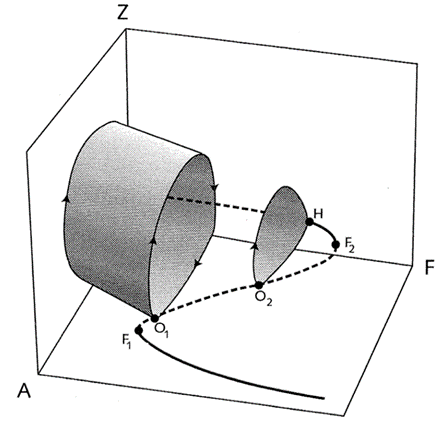
Fig. 4. 3D Bifurcation Illustrating Ecological Stability. This diagram depicts the impact of fish predation on the dynamic equilibria within an aquatic ecosystem. The absence of a limit cycle, which is typically found between homoclinic bifurcations (denoted O1 and O2), indicates a disruption in predator-prey interactions. This is caused by a collision with the saddle point H, which is crucial for defining the boundaries of the attraction basin that determines stable algal populations. The axes labeled A, F, and Z represent different system parameters or states that affect algal dominance (Scheffer et al., 1997).

In addition to the previously shown model of plankton dynamics, the seasonal changes, primarily light, temperature, and fish predation that influence their dynamic relationship are also accounted for. This is modeled by imposing a sinusoidal variation on key parameters throughout the year. Light plays a crucial role in setting the upper limit for algal biomass, leading to the assumption that the carrying capacity for algae, denoted as K, is a direct function of light availability (Scheffer et al., 1997). Simultaneously, temperature significantly impacts the metabolism of both algae and zooplankton, influencing their growth rate (r), grazing rate (g), mortality (m), and the intensity of fish predation (F) (Scheffer et al., 1997). To encapsulate the effect of seasons, each of these parameters is modified by a seasonal impact, shown in Equation 7, a periodic function of time with t = 0 representing January 1^st (Scheffer et al., 1997). The model simplifies the minimum and maximum values of these parameters by relating them to a factor $\frac{1-e}{1+e}$ , where ε represents the amplitude of seasonal forcing (Scheffer et al., 1997).

$\sigma(t) = \frac{1-\varepsilon \cos\left(\frac{2\pi t}{365}\right)}{1+\varepsilon}$

Equation 7: Seasonal impact (Scheffer et al., 1997).

$\frac{dA}{dt} = \sigma(t) rA\left(1 - \frac{A}{\sigma(t) K}\right) - Z\sigma(t) g \frac{A}{A+h_A} + d(\sigma(t) K - A)$

$\frac{dZ}{dt} = e\sigma(t) gZ \frac{A}{A+h_A} - \sigma(t) mZ - \sigma(t)^2 F \frac{Z^2}{Z^2 + h_Z^2}$

Equation 8: Differential equations that model the stable equilibria and limit cycles of Daphnia’s system dynamics (Scheffer et al., 1997).

Notably, fish predation undergoes considerable seasonal variation due to the reproductive cycle of planktivorous fish. The springtime growth of young fish leads to an augmented predation pressure on zooplankton, peaking in summer. This additional factor is incorporated by multiplying the fish predation parameter F with an extra seasonal impact ρ.

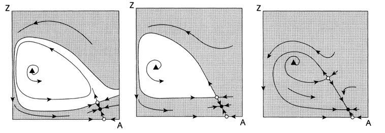
Fig. 5. Phase portraits showing effects of increasing fish predation pressure F with A as algal populations and Z as herbivorous zooplankton: The triangle indicates the unstable equilibrium, central to the limit cycle. Open circles represent the trivial equilibrium of only algae and the positive saddle point, while the filled circle signifies the stable “turbid equilibrium” described in the text. The grey area marks the attraction basin for the turbid equilibrium. a) Two attractors scenario (a cycle and turbid equilibrium) separated by the stable manifold of a saddle, also known as separatrix; b) Single attractor scenario (turbid equilibrium) with the cycle making homoclinic contact with the saddle; c) Sole global attractor scenario featuring the turbid equilibrium (Scheffer et al., 1997).

Behavioral adaptations during algal bloom

In this trophic relationship, Daphnia have also developed a remarkable behavioral adaptation to cope with the variability in phytoplankton size: they can adjust the gap between their carapace valves (Gliwicz & Siedlar, 1980). High concentrations of phytoplankton trigger Daphnia to narrow this gap, selectively filtering out larger algal forms that are less efficient for food collection and ingestion (Gliwicz & Siedlar, 1980). This is not a chemical but a mechanical response, aimed at optimizing the size of particles collected, albeit at the expense of their overall feeding rate. Large or filamentous algae, while initially seeming to hinder Daphnia‘s feeding, do not necessarily preclude their use as a food source (Gliwicz & Siedlar, 1980). In fact, Daphnia can ingest these larger phytoplankton forms, as evidenced by the remains found in their gut contents, particularly in oligotrophic lakes where food is scarce (Gliwicz & Siedlar, 1980). Furthermore, Daphnia can thrive on a diet of dense cultures of large algae like Anabaena filaments (Gliwicz & Siedlar, 1980). This suggests that Daphnia can manage large, hard-to-digest algae either when they are encountered infrequently or when they are so abundant that they become the primary, though not optimally utilized, food source (Gliwicz & Siedlar, 1980). The ability to narrow the carapace gape is thus a crucial survival strategy for Daphnia during summer algal blooms, allowing them to maintain nutritional intake even when their preferred food size is limited (Gliwicz & Siedlar, 1980).

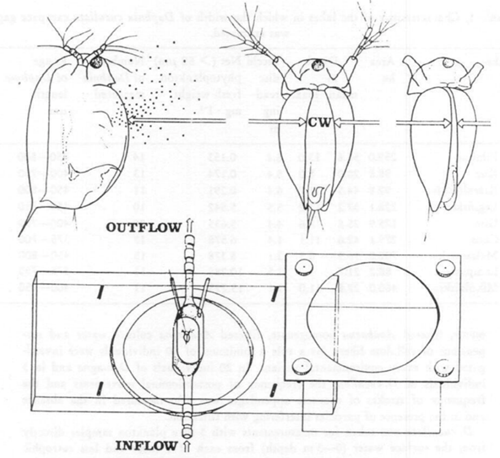
Fig. 6. Lateral and ventral views of Daphnia magna illustrating the area of carapace for water and food suspension to flow into the filtering chamber and showing where the width of the gape (CW) was measured (top) and (bottom) general view of flow chamber with Daphnia fixed to the end of a capillary (Gliwicz & Siedlar, 1980).

Chaoborus phantom midge

Chaoborus remain motionless in the water column using their two pairs of tracheal air sacs, which allows them to subtly position themselves for an attack. Their interaction with prey is largely determined by the vertical distribution and swimming speed of their prey, such as Daphnia, as well as the vertical positioning of the Chaoborus. They are equipped with setae lining their bodies, which are sensitive to the approach of prey and upon detection, they execute a rapid striking motion with their prehensile antennae. Prey not wider than the Chaoborus‘ mouth gape is swallowed whole, while larger prey often manages to escape (Hanazato, 1991).

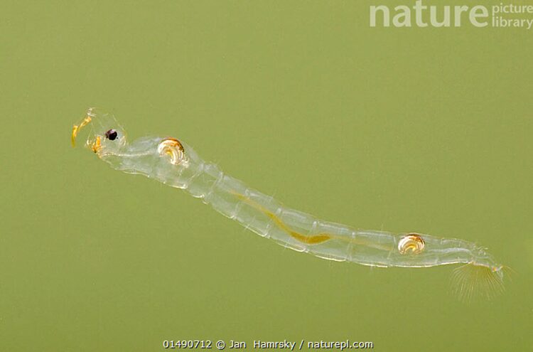
Fig. 7. Chaoborus Phantom Midge (Flavicans) (Hamrsky, 2015)

The defensive strategies of Daphnia include changes in life history traits, such as a shift towards larger body sizes at first reproduction and the production of fewer but larger offspring during periods of danger. Additionally, Daphnia develop protective spines and engage in antipredator behaviors, notably upward migration during daytime to avoid Chaoborus since they typically prefer darker, deeper waters. The cost-benefit analysis of these defenses was evaluated by comparing growth rates in Daphnia populations in both control and kairomone-exposed environments. The costs of these defenses vary from a decrease in population growth by 48.4 %, suggesting that Daphnia populations fared better in the presence of predator kairomone, to a substantial increase in cost of up to 153.3 %, indicating a significant investment in predator defense. Over a 10-day period, the overall cost of these defenses averaged 32.3 %. Despite these costs, there was no significant change in the number of eggs produced per ovigerous female. However, by the tenth day, there was a marked decrease in the percentage of adult females that were ovigerous in the kairomone and predation treatments, as compared to the control group. This indicates a reproductive cost associated with the defense mechanisms (Hanazato, 1991).

The benefits of these defensive strategies also showed great variety. At one end, there was a perceived negative benefit of 146.8 %, suggesting that predation could paradoxically benefit the Daphnia populations while the benefit was as high as 68.4 %, indicating a strong advantage in developing these defenses against predation. The defensive strategies adopted by Daphnia demonstrate a complex balance of costs and benefits impacting their population growth. Knowing that defenses against Chaoborus leads to a significant reduction of 32.3 % in Daphnia population growth, which is highlighted when comparing the kairomone-treated populations with control groups, those in control conditions exhibited higher growth rates and reached maximum densities more quickly. The decline in growth rate among kairomone-exposed Daphnia is attributed primarily to their induced antipredator defenses (Hanazato, 1991).

Elaborating further on the behavioral upward migration during the day, while a strategy to evade Chaoborus, brings Daphnia into environments with different challenges. Notably, the warmer temperatures in shallower waters can negatively impact larger-bodied Daphnia, as they might face energy limitations. Additionally, this upward migration results in increased competition for food. As they congregate in the upper layers of the water column, there is greater competition due to the reduced volume of habitat and available resources. This heightened competition for food is detrimental to the Daphnia population at times than the direct predation by Chaoborus. Other costs include a potential decrease in feeding rates, either due to the presence of their kairomone or the chemical cues associated with crowding. This reduction in feeding rate could further hamper somatic growth rates (Hanazato, 1991).

Moreover, there was a significant drop in the percentage of females producing eggs, possibly due to such competitive conditions, despite the number of eggs per ovigerous female remaining constant. Another cost factor is the exposure to UV radiation since the migration of Daphnia upwards in response to Chaoborus kairomone during the day results in higher levels of harmful UV radiation. This exposure has the potential to adversely affect both the survival and reproductive success of Daphnia. However, the development of protective spines, particularly on the dorsal lower margin of the head (neck spines) in younger Daphnias, stands out. These spines have been shown to increase the escape rate from Chaoborus attacks by up to 60 %, significantly enhancing the chances of survival for these juveniles (Young & Riessen, 2005) (Boeing et al., 2005).

Swimming behavior

As they live in aquatic environments, Daphnia exhibit specialized swimming behaviors. These can be impacted by different elements like predator cues (kairomones) that are found in the water and used by Daphnia for various adaptations like it was seen in previous papers (1,2) (Watt & Young, 1994).

Normal swimming behavior

In normal water conditions (no kairomones or chemicals), a study found that the swimming patterns depend on the Daphnia species that is studied as it can be seen in Figure 8.

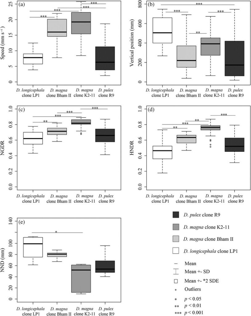
Fig. 8. Swimming behavior of Daphnia in regular water. a) shows the average speed of the different Daphnia species, b) shows the vertical position of the organisms, c) shows the net growth displacement ratio (NGDR) which is the motion patterns of Daphnia in terms of the turning behavior, d) shows the horizontal net displacement ratio (HNDR) which is also a motion pattern parameter but with the horizontal direction change and e) corresponds to the swarming behavior which is measured in nearest-neighbour distance (Langer et al., 2019).

What can be taken away from the data in Figure 8 is that D. magna swims the fastest. It is believed that larger daphniid species swim faster which correlates with the above data since D. magna is the largest out of all Daphnia species. This is also believed to be the case in individuals from a species. In fact, if we look at two individuals from the same species, the largest one will likely swim faster. Other than that, no correlation can be seen in swimming behavior for Daphnia swimming in normal conditions (Langer et al., 2019).

Special swimming behavior

As it was seen in a previous essay (Daphnia’s Chemical Interactions: Varying Conditions Require Varying Responses and Phenotypic Adaptation of Daphnia Throughout Evolution), kairomones have an effect on Daphnia‘s swimming behavior. An effect of kairomones on swimming behavior that was not presented in the previous papers was reduced swimming speed in the presence of predators. Something that could explain this effect is that reducing swimming speed would make Daphnia harder to detect by visual predators. Also, by swimming at a lower speed, they would also save energy and use some of that saved energy to become more alert to their surroundings. Also, it was shown that their vertical position would get lower when in the presence of kairomone. Also mentioned in previous papers is the swarming behavior of Daphnia. However, a nuance that could be added is that swarming does not happen in all population sizes. In fact, during a study, researchers found that the organisms they used did not exhibit such behavior. In fact, the Daphnia that were exposed to fish kairomones during the study were even found to disperse in the water body. An interesting hypothesis on why that happened is that Daphnia‘sadaptations may depend on population density. In fact, in the wild, they live in populations constituted of numerous individuals which, while in the lab, was not the case. Therefore, swarming would not be an ideal behaviour as they would be more easily consumed by their predator. Therefore, Daphnia could be aware of the size of their group and adapt accordingly. Similar behavior was seen for Notonecta– and Chaoborus-induced behavior, but it was less dramatic. The results of the study can be found in Figure 9 (Langer et al., 2019).

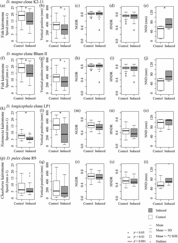
Fig. 9. a)-e) shows the effect of fish kairomone on speed, vertical position, turning behavior (NGDR), horizontal direction change (HNDR) and distance from nearest individual (NDD) on D. magna, comparing the control to the induced clone. In f)-j), the same parameters are evaluated to compare a control and an induced D. magna but another clone. In k)-o), the same parameters are evaluated to compare a control and an induced Daphnia longicephala but with Notonecta kairomone. In f)-j), the same parameters are evaluated to compare a control and an induced D. pulex but another Chaoborus kairomone. The predator/prey relations were chosen by the people who conducted the studies but were not explained (Langer et al., 2019).

Another impact of kairomone detection is that Daphnia will do horizontal migration. However, this depends on the predator Daphnia is trying to avoid. In fact, a study calculated the predation risk (PRI) associated with the space occupied by a Daphnia and realized that when they were in open water, the PRI was higher for Chaoborus, but when they were close to the shore, in the vegetation, the PRI was higher for Ischnura. This is obviously related to where the two species live, but a question subsists: where could Daphnia go to be safe? Scientists performed experiments to calculate the PRIs in different systems using the following formula:

$PRI_{i,j} = N(CH)_{i,j} \times PR(CH)_{i,j} + N(IS)_{i,j} \times PR(IS)_{i,j}$

Equation 9: Where PRI is the predation risk, the PRs are the predation rates (per capita predation rate per unit of surface area) and the Ns are the average number per aquarium surface area of the predators that were present during the experience. The CH’s relate to Chaoborus and the IS’s to Ischnura. The i’s and the j’s are related to the microhabitat (i) and predator treatment (j) used in the experiment as they were varying. Therefore, those are more related to how it was performed, but the most important is to get a general idea of how the PRIs were calculated (Meutter et al., 2005).

Therefore, the number of Daphnia in open water depends largely on both predators. The study also found that it depended on time. What was expected happened during the study: when there is only the Chaoborus species present, less Daphnia are present in open water than when both Ischnura and Chaoborus are there. When there is Ischnura only, Daphnia tend to only stay in open waters as it can be seen in Figure 10 (Meutter et al., 2005). A conclusion that can be made from that is that Daphnia‘s natural occupied space in the water is most likely open water and they would only go to the littoral when the Chaoborus phantom midge larvae is present (Meutter et al., 2005).

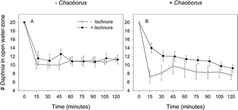
Fig. 10. This figure shows the number of Daphnia in open water depending on the treatment they were submitted to (presence or absence of Ischnura and Chaoborus) (Meutter et al., 2005).

Hence, the number of Daphnia seems to stabilize after some time as they would know where the predators are. The same study also calculated the predation risk using the previously shown formula and the following results were obtained:

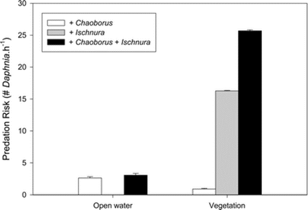
Fig. 11. This figure shows the predation risk associated with the different types of predators and the zone (Meutter et al., 2005).

The figure above explains why Daphnia can move to vegetation zones, but they never actually enter them. In fact, it would be the best thing as they would have the highest chances of avoiding Chaoborus but also not get face-to-face with Ischnura. This can also be caused by the fact that in shallow lakes, Chaoborus only have a small preference for open-water zone (58-65 %). Therefore, Daphnia will prefer the open water, but still flee it to escape from Chaoborus, while still watching out for Ischnura (Meutter et al., 2005).

Conclusion

As explained in this paper, the many interactions of Daphnia with its environment and other organisms may be modelled to demonstrate how they have been optimized. Through logic and mathematics, many design solutions can be found through water fleas’ interactions, position, morphology and even reproduction. First, because both types of reproduction can have their advantages (asexual leads to high population growth and sexual to genetic diversity), Daphnia have found the best of both worlds by doing cyclical parthenogenesis and being able to achieve multiple types of reproduction depending on the environmental conditions, practicing asexual reproduction to populate a new environment or when there are many predators, but still being able to assure genetic diversity. Furthermore, no new design solutions were exposed with game theory. However, some design solutions (cyclical parthenogenesis and phenotypic plasticity, explained in previous papers (Daphnia’s Chemical Interactions: Varying Conditions Require Varying Responses and Phenotypic Adaptation of Daphnia Throughout Evolution) were proven to be useful with that theory as they propose advantages. Furthermore, behavioral adaptations to their carapace are seen during algal bloom, which aids Daphnia in being able to optimize their algae intake. Furthermore, when being exposed to Chaoborus kairomone, on top of showing morphological changes, Daphnia may also delay their reproduction. Even though that could be seen as negative, this shows how important phenotypic plasticity is since its advantages outweigh the consequences of delaying reproduction. To continue, many design solutions are found in their swimming behaviors, when exposed to kairomones. In fact, a reduced swimming speed was observed when Daphnia were exposed to predatory cues. This is used to make them less detectable by predators. Also, on top of performing diel vertical migration to escape their predators, Daphnia also perform horizontal migration. This process is based on multifactorial predation and depends on the presence of predators that are in more than one zone. The predation risks need to be analyzed in both places to know which is the safest for water fleas. Moreover, Daphnia‘s swimming pattern and survival strategies are also dependent on the size of their population. In fact, they would only swarm when in big groups as this is when it is optimal to do so.

Overall, over the past papers, the biggest takeaway on Daphnia, showing how well they evolved to be the fittest possible is their extremely fast adaptation to their environment. Whether it is biotic or abiotic factors, Daphnia have a solution for a wide range of ecological problems. Briefly, water fleas are masters of morphosis.

References

Boeing, W. J., Wissel, B., & Ramcharan, C. W. (2005). Costs and benefits of Daphnia defense against Chaoborus in nature. Canadian Journal of Fisheries and Aquatic Sciences, 62(6), 1286-1294. https://doi.org/10.1139/f05-043

Boersma, M. (1997). Offspring size and parental fitness in Daphnia magna. Evolutionary Ecology, 11(4), 439-450. https://doi.org/10.1023/A:1018484824003

Choi, T. J., Han, S. M., Malik, A., & Kim, C. B. (2023). Comparative transcriptome analysis of two Daphnia galeata genotypes displaying contrasting phenotypic variation induced by fish kairomones in the same environment of the Han River, Korea. BMC Genomics, 24(1), 580. https://doi.org/10.1186/s12864-023-09701-x

Decaestecker, E., De Meester, L., & Mergeay, J. (2009). Cyclical Parthenogenesis in Daphnia: Sexual Versus Asexual Reproduction. In I. Schön, K. Martens, & P. Dijk (Eds.), Lost Sex: The Evolutionary Biology of Parthenogenesis (pp. 295-316). Springer Netherlands. https://doi.org/10.1007/978-90-481-2770-2_15

Ebert, D. (2022). Daphnia as a versatile model system in ecology and evolution. Evodevo, 13(1), 16. https://doi.org/10.1186/s13227-022-00199-0

Einum, S., Ullern, E. R., Walsh, M., & Burton, T. (2022). Evolution of population dynamics following invasion by a non-native predator. Ecology and Evolution, 12(9), e9348. https://doi.org/https://doi.org/10.1002/ece3.9348

Exponential & logistic growth. Khan Academy. Retrieved November 29 from https://www.khanacademy.org/science/ap-biology/ecology-ap/population-ecology-ap/a/exponential-logistic-growth

Genkai-Kato, M. (2004). Nutritional value of algae: a critical control on the stability of Daphnia–algal systems. Journal of Plankton Research, 26(7), 711-717. https://doi.org/10.1093/plankt/fbh069

Gliwicz, Z., & Siedlar, E. (1980). Food size limitation and algae interfering with food collection in Daphnia. Arch. Hydrobiol., 88, 155-177.

Goitom, E., Kilsdonk, L. J., Brans, K., Jansen, M., Lemmens, P., & De Meester, L. (2018). Rapid evolution leads to differential population dynamics and top-down control in resurrected Daphnia populations. Evol Appl, 11(1), 96-111. https://doi.org/10.1111/eva.12567

Hammerstein, P., & Selten, R. (1994). Chapter 28 Game theory and evolutionary biology. In Handbook of Game Theory with Economic Applications (Vol. 2, pp. 929-993). Elsevier. https://doi.org/https://doi.org/10.1016/S1574-0005(05)80060-8

Hamrsky, J. (2015). Phantom midge (Chaoborus flavicans) larva, Europe, February, controlled conditions. Nature picture library. Retrieved December 2 from https://www.naturepl.com/stock-photo-phantom-midge-chaoborus-flavicans-larva-europe-february-controlled-image01490712.html

Hanazato, T. (1991). Effects of a Chaoborus-released chemical on Daphnia ambigua: Reduction in the tolerance of the Daphnia to summer water temperature. Limnology and Oceanography, 36(1), 165-171. https://doi.org/https://doi.org/10.4319/lo.1991.36.1.0165

Huttegger, S. M., & Zollman, K. J. S. (2013). Methodology in Biological Game Theory. The British Journal for the Philosophy of Science, 64(3), 637-658. https://doi.org/10.1093/bjps/axs035

Kankala, P. (1988). The relative importance of algae and bacteria as food for Daphnia longispina (Cladocera) in a polyhumic lake. Freshwater Biology, 19(3), 285-296. https://doi.org/https://doi.org/10.1111/j.1365-2427.1988.tb00351.x

La, G. H., Choi, J. Y., Chang, K. H., Jang, M. H., Joo, G. J., & Kim, H. W. (2014). Mating behavior of Daphnia: impacts of predation risk, food quantity, and reproductive phase of females. PLoS One, 9(8), e104545. https://doi.org/10.1371/journal.pone.0104545

Langer, S. M., Weiss, L. C., Ekvall, M. T., Bianco, G., Hansson, L.-A., & Tollrian, R. (2019). A three-dimensional perspective of Daphnia’s swimming behavior with and without predator cues. Limnology and Oceanography, 64(4), 1515-1525. https://doi.org/https://doi.org/10.1002/lno.11132

Maynard Smith, J. (1972). On evolution / John Maynard Smith. Edinburgh University Press.

McCauley, E., Nisbet, R. M., Murdoch, W. W., de Roos, A. M., & Gurney, W. S. C. (1999). Large-amplitude cycles of Daphnia and its algal prey in enriched environments. Nature, 402(6762), 653-656. https://doi.org/10.1038/45223

McNamara, J. M., & Leimar, O. (2020). Game Theory in Biology: concepts and frontiers. Oxford University Press. https://doi.org/10.1093/oso/9780198815778.001.0001

Meutter, F. V. d., Stoks, R., & Meester, L. D. (2005). Spatial avoidance of littoral and pelagic invertebrate predators by Daphnia. Oecologia, 142(3), 489-499. https://doi.org/10.1007/s00442-004-1738-5

Nash, J. F. (1950). Equilibrium points in <i>n</i>-person games. Proceedings of the National Academy of Sciences, 36(1), 48-49. https://doi.org/doi:10.1073/pnas.36.1.48

Palamara, G. M., Dennis, S. R., Haenggi, C., Schuwirth, N., & Reichert, P. (2022). Investigating the effect of pesticides on Daphnia population dynamics by inferring structure and parameters of a stochastic model. Ecological Modelling, 472, 110076. https://doi.org/https://doi.org/10.1016/j.ecolmodel.2022.110076

Scheffer, M., Rinaldi, S., Kuznetsov, Y. A., & van Nes, E. H. (1997). Seasonal Dynamics of Daphnia and Algae Explained as a Periodically Forced Predator-Prey System. Oikos, 80(3), 519-532. https://doi.org/10.2307/3546625

Sinko, J. W., & Streifer, W. (1967). A New Model For Age-Size Structure of a Population. Ecology, 48(6), 910-918. https://doi.org/10.2307/1934533

Smith, F. E. (1963). Population Dynamics in Daphnia magna and a New Model for Population Growth. Ecology, 44(4), 651-663. https://doi.org/10.2307/1933011

Stoeckel, J., & Siriwardena, S. (2022). Daphnia (water flea) (Vol. CABI Compendium). CABI. https://doi.org/10.1079/cabicompendium.102727

Tagg, N. (2004). The ecological cost of sexual reproduction

Watt, P. J., & Young, S. (1994). Effect of predator chemical cues on Daphnia behaviour in both horizontal and vertical planes. Animal Behaviour, 48(4), 861-869. https://doi.org/https://doi.org/10.1006/anbe.1994.1310

Young, J. D., & Riessen, H. P. (2005). The interaction of Chaoborus size and vertical distribution determines predation effects on Daphnia. Freshwater Biology, 50(6), 993-1006. https://doi.org/https://doi.org/10.1111/j.1365-2427.2005.01381.x