A Mathematical Approach to Understanding Volvox

Robinson Libman, Meryem Louni, Ryan McGibbon, Ali Najjar

Abstract

This paper sheds light on the suitability of mathematical theories and models to unveil a variety of design solutions inherent to Volvox. Having evolved from the unicellular Chlamydomonas, Volvox demonstrates that multicellularity is of particular interest to improve the nutrient uptake per somatic cell. Also, randomness plays a role in the self-assembly of cells in an almost perfect spherical shape which has the lowest fractal dimension, making it energetically ideal. Moreover, modeling of the colony’s motion highlighted that the species’ swimming technique is remarkably effective in their low Reynolds number environments. Finally, a mathematical approach of Volvox’s inversion facilitates the understanding of this complex process. All in all, the extraordinary properties of this microorganism both provide an insight into the driving forces behind multicellularity, and inspiration for biomimicking innovations.

Introduction

The multicellular freshwater green algae Volvox consists of a colony of 500 to 50,000 cells and is a fascinating organism to study (Umen & Herron, 2021). Volvox has many parallels to higher-level organisms making it the ideal algae to study in order to gain a deeper understanding of many functions within these higher-level organisms. But more importantly, the transition from unicellular to multicellular organisms could not be made easier to analyze than with Volvox, given its quite recent deviation from its unicellular counterpart, Chlamydomonas reinhardtii, about 200 million years ago (Umen & Herron, 2021). It is interesting to observe what was required of the colony to adapt to its multicellular lifestyle, what morphological aspects had to be changed, what new functions had to be implemented for the larger colony to function and thrive.
The beauty of Volvox lies in the modelling and simulations that arise from studying various aspects of its lifestyle. In this paper, we shall attempt to provide a more abstract, mathematical analysis of this amazing microorganism. We shall dive back within the colony, this time to analyze the complexity lying within its simplicity, something that can only be understood through nature’s marvelous concept of fractals, and we shall touch upon the scaling laws present throughout Volvox’s evolution, as well as the randomness of its self-assembly. Then, we shall revisit the physical phenomena governing the colony’s lifestyle with mathematical models, both for describing Volvox’s swimming and motility, and for the driving forces behind both types of its embryo inversion. As always, we shall consider the various design solutions Volvox uses to optimize its way of living to once again prove the sheer ingenuity hidden within this tiny marvel of a multicellular organism.

Fractals: studying volvox complexity

Tree branches, snowflakes, lightning, and even the inside of our lungs all have a similar property: that of order within chaos. Indeed, while these patterns found in nature seem to be governed by pure randomness, there is a level of organization hidden within them, which is expressed through the idea of self-similarity. When looking at a tree (see Fig. 1), one can zoom into the branches and observe that the pattern seems to repeat itself, at smaller and smaller scales. Of course, we do reach a limit where the branches don’t subdivide further, demonstrating that these patterns are, like all things in nature, finite. However, this idea of self-similarity can be thought of in a more general way by considering the concept of fractals. Fractals are complex shapes often associated with structures that are detailed at all scales and that generally tend to demonstrate repeating patterns as one zooms into them. An important feature that separates fractals from shapes typically considered in conventional geometry, often characterized as Euclidean geometry, is the fact that fractals don’t have an integer dimension (Pham & Musielak, 2023). Yes, there is such a thing as a 1.585-dimensional shape, which we shall cover soon. But first, a more important question must be answered: how is this concept possibly related to Volvox?

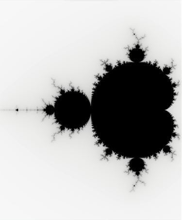
The Mandelbrot set is one of the most famous fractals out there. It is generated by recursively running the function $z_{n+1} = z_n^2 + c$ and plotting the points that converge after a certain number of iterations in the complex plane. This is a purely mathematical fractal that can be infinitely zoomed into. Here’s an amazing video of a Mandelbrot zoom.

Fig. 1. Self-similar patterns in nature (From Sigma Documentaries (2021) & Adobe Stock).

Volvox fractals

Looking at an image of Volvox, like in Fig. 2 below, you may already start to see how the concept of self-similarity is indeed present within them. Volvox colonies consist of two types of cells: gonidia (germ cells) and somatic cells (Umen, 2020). While there are thousands of somatic cells, there are only a couple gonidia, which are much larger (Umen, 2020). Within these gonidia forms a new, smaller colony. Indeed, at the end of the Volvox life cycle, the gonidia are released from the larger colony through a process of inversion and form new juvenile colonies, which shall be discussed later in this paper. In other words, we have spherical colonies within a larger spherical colony, which means that we can indeed observe some level of self-similarity within Volvox. Given that this self-similarity is of course finite, if we were to evaluate the fractal nature of Volvox or other green algae, we would need a slightly modified definition of fractals. Pham and Musielak (2023), whose intentions were in fact to observe green algae through the lens of fractals, came up with the concept of “reduced fractals”. Its definition is similar to that of regular fractals but takes into account those with limited ranges of self-similarity and magnification (Pham and Musielak, 2023). Volvox as fractals, despite their finite magnification, may be used to measure complexity, especially in biological systems, which can provide a deeper understanding of how complex these colonies truly are.

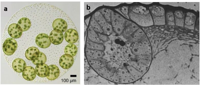
Fig. 2. (a) A picture of a whole Volvox carteri colony in which the gonidia (green circles within the colony) are developing and forming a smaller colony within them (Adapted from Umen (2020)). (b) A more zoomed in look at a gonidium (large circular shape on the left) where we can see the same chain of somatic cells forming within the inside edge of the gonidium as within the edge of the larger colony (Adapted from Kirk et al. (1986)).

Fractal geometry

Typically, when considering geometry, we think of lines, curves, areas, and volumes. We think of smooth lines, where curves are continuous and differentiable, and if they don’t appear smooth, they will eventually appear as such if we zoom in enough. This is known as Euclidean geometry (Kenkel & Walker, 1996). In the context of biology, we see conifers as cones, their trunks as cylinders, and their branches as one-dimensional broken lines. But consider the following analogy inspired by Kenkel and Walker (1996): a small insect, about 1 cm in size, wants to travel around the circumference of the previously mentioned tree trunk. One could say that it will travel 2πr meters, with r being the radius of the trunk. However, this insect will have to travel a much larger distance, because the surface of the trunk is far from smooth. The roughness of the bark creates many bumps and wells that the insect will have to overcome. Now consider an even smaller insect, about 1 mm in size. It will have to travel an even greater distance, as we have scaled down our perspective and are faced with more bumpy terrain that was not a concern at the scale of the first insect. By this logic, the circumference of the trunk would tend to infinity as we zoom to smaller and smaller scales. While this is indeed the outcome of purely mathematical fractals, we once again come across the constraint of things being finite in real life, so the circumference is technically not truly infinite. Nevertheless, that doesn’t make finding the true circumference or cross-sectional area of the trunk any easier. Calculus cannot explain this relation, so we must therefore refer to fractal geometry.

The fractal dimension

Benoit Mandelbrot, the father of fractals, the man who came up with the word and popularized the idea, figured out a way of characterizing fractal geometry through what is called fractal dimensions (Pham & Musielak, 2023). They are a measure of the complexity of a fractal, or really of any geometric figure by assigning a typically non-integer dimension to it. Funnily enough, this implies that regular geometry involving 1D, 2D, or 3D shapes is actually a special case of fractal dimensions where the dimension is an integer. Essentially, the fractal dimension is a measure of how fast detail grows with increasing magnification, and is given by the formula:

$FD = \frac{\log(N)}{\log(r)}$

where FD is the fractal dimension and N represents the number of distinct copies of the original shape in the magnification level r (Pham & Musielak, 2023). Let us look at an example involving a simple 2-dimensional shape first. A square can be split into 4 identical pieces that are self-similar to the original square but smaller by a factor of 2 (see Fig. 3). This means that N=4 and r=2. Plugging this into equation (1), we have: $FD = \frac{\log(4)}{\log(2)} = \frac{\log(2^2)}{\log(2)} = \frac{2\log(2)}{\log(2)} = 2$ , so we obtain a dimension of 2, which is exactly as expected. Looking at a cube, we can split it into 8 identical pieces self-similar to the original, also scaled down by a factor 2 (again, refer to Fig. 3). The dimension is therefore: $D = \frac{\log(8)}{\log(2)} = \frac{\log(2^3)}{\log(2)} = \frac{3\log(2)}{\log(2)} = 3$ , and a cube is indeed a 3-dimensional shape. But what about the Sierpinski triangle? This fractal can be split into 3 self-similar identical shapes scaled down by a factor of 2 (Fig. 3). This would mean that the fractal dimension is: $FD = \frac{\log(3)}{\log(2)} \approx 1.585$ . The Sierpinski triangle is therefore 1.585-dimensional! For a more in-depth explanation of fractal dimensions, refer to this video by 3Blue1Brown (2017).

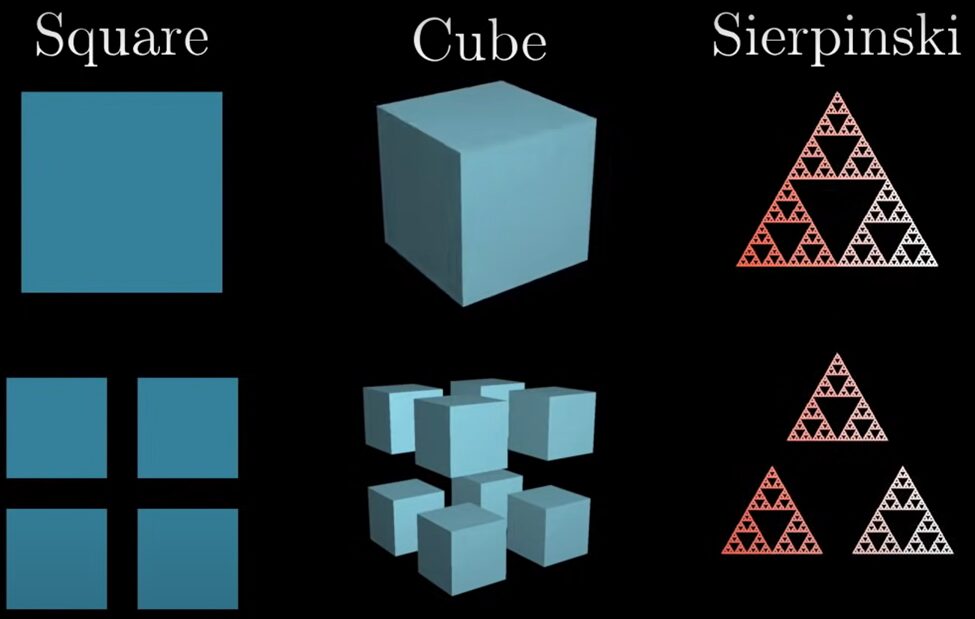
Fig. 3. Visualization of how a square, cube, and Sierpinski triangle can be split into equal parts self-similar to the original shape and scaled down by a factor 2 (3Blue1Brown, 2017).

Now, the previous examples are ones that can go on to infinity, to smaller and smaller magnifications. They are also shapes that are purely self-similar at all scales. That is not really the case in nature. We already know that fractals in nature are finite, and none are purely self-similar, as there is always a level of randomness and irregularity to them. This is why approximations must be made to find the fractal dimension of naturally occurring shapes. A technique that is often used to find the fractal dimension of certain shapes, and the one used by Pham and Musielak (2023) to measure the fractal dimension of Volvox, is the box-counting method. This involves placing the shape, which in the case of the researchers is a picture of the alga they are studying, in a grid and counting the number of boxes of the grid the shape fills. As the grid becomes finer and finer, with smaller and smaller boxes, one can find that the number of boxes N scales proportionally to the change in magnification level r raised to the dimension of the fractal DF. In other words, if we start with a number of boxes c, we can obtain the following relation between N and r:

$N = c \cdot r^{FD} \iff \log(N) = \log(c) + FD \cdot \log(r)$ .

This implies that if we plot log⁡N as a function of log⁡r, the fractal dimension would correspond to the slope! This concept is once again explained very well in the video by 3Blue1Brown (2017). Since the purpose of measuring fractal dimensions is to evaluate the complexity of the shape, Pham and Musielak (2023) were able to approximate and compare complexities of different algae, including Volvox, using this method, though they also added a gray level to each box of the grid to designate details within the patterns of the studied algae.

Are volvox truly “complex”?

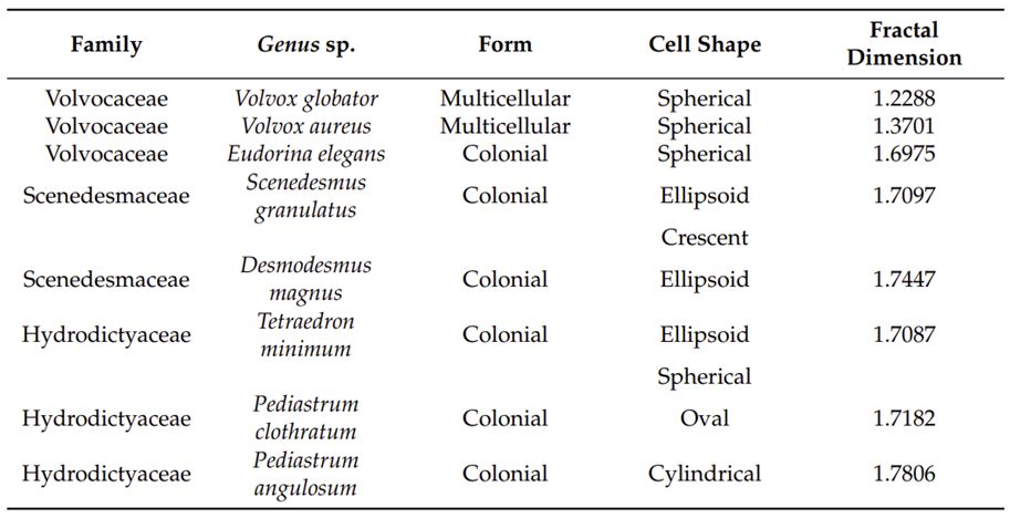
Figures 4 and 5 show images of the 17 algae studied by Pham and Musielak (2023) and tables 1 and 2 show the obtained fractal dimensions. The researchers observed that the two Volvox species they studied had the lowest fractal dimensions, with Volvox globator (Fig. 5a) having a dimension of 1.2288 and Volvox aureus (Fig. 5b) having one of 1.3701. Note that these were the only two multicellular green algae studied in this paper and the other species were all colonial or unicellular, with the latter having the species with the highest fractal dimensions. Does this mean that Volvox are the least complex among all these species? Is this data saying that multicellular organisms are less complex than unicellular ones? Well, not quite. Pham and Musielak (2023) have in fact stated that Volvox are the most complex among the algae that were studied. Then why the lower values?

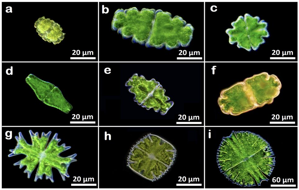
Fig. 4. Images of unicellular green algae of the class Zygnematophyceae. (a) Euastrum bidentatum, (b) Euastrum oblongum, (c) Euastrum verrucosum, (d) Euastrum ansatum, (e) Euastrum humerosum, (f) Euastrum crassum, (g) Micrasterias americana, (h) Micrasterias truncate, and (i) Micrasterias rotata (Pham & Musielak, 2023).

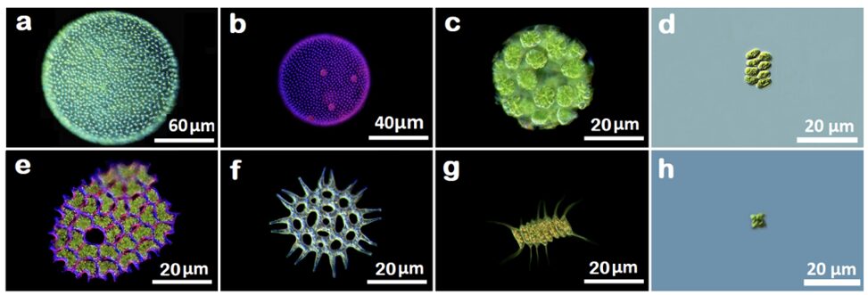
Fig. 5. Images of colonial and multicellular green algae of the class Chlorophyceae. (a) Volvox globator, (b) Volvox aureus, (c) Eudorina elegans, (d) Scenedesmus granlulatas, (e) Pediastrum clothratum, (f) Pediastrum angulosum, (g) Desmodesmus magnus, and (h) Tetraedron minimum (Pham & Musielak, 2023).

Table 1 Fractal dimension of the algae from Fig. 4. (Pham & Musielak, 2023).

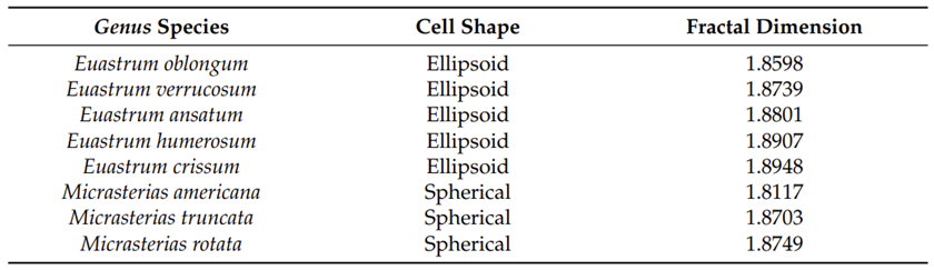
Table 2 Fractal dimension of the algae from Fig. 5. (Pham & Musielak, 2023).

Volvox show more order and organization, since they are multicellular organisms that show cellular differentiation, which can be seen visually, with the spheres representing the gonidia neatly contained within the larger sphere of the colony, and with the somatic cells equally distributed around the sphere. This cellular differentiation allows for splitting of the tasks of the organism, and the large quantity of somatic cells allows for less load and dependance on each one of them. This smarter division and distribution of tasks shows that an organism does not have to be extremely “complex-looking” to truly be complex, and really demonstrates the vague nature of the word “complex” itself. Asymmetric organisms are often considered the least complex organisms, as there is no semblance of organization, though their shape definitely “looks” more complex than some more advanced, symmetrical organisms. An important element to note is that these fractal dimensions were calculated based on simple 2-dimensional images of these organisms. If one were to analyze the fractal dimension of the true 3-dimensional model of these algae, they would most likely find that Volvox would have a higher fractal dimension in that regard, as they would have much more depth and self-similar patterns than the other relatively flat creatures.
While the aim of Pham and Musielak (2023) was to present a new method of classifying species within their families using fractal dimensions and taking green algae as an example, they nevertheless were able to provide a mathematical analysis of the complexity of Volvox, showing that looks and levels of complexity are not necessarily related. Then what was the point of all this? Well, one important observation from their calculated values is that the gap between the fractal dimension of Volvox and other colonial organisms is much larger than the gap between colonial and unicellular organisms, showing that Volvox made quite a substantial leap in evolution by being a multicellular organism, as their structure is much more different than the previous colonies who have fractal dimensions of 1.7 and above. Interestingly, Pham and Musielak (2023) were also able to show a trend of spherical shapes for algae providing by far the lowest fractal dimensions, beating oval, cylindrical or ellipsoidal shapes. This implies that a spherical shape is ideal, as it is the simplest of them all.
As mentioned at the beginning of this section, fractals are the order that is found within the chaos of nature, yet organisms that demonstrate greater organization could also present less complex fractals. A possible explanation for this is that nature favours simplicity and order over anything as it optimizes energy usage, but it does not prevent it from experiencing the randomness of the Universe. Fractals are within every one of us, in our lungs, in our nervous system, they are within Volvox, and they are within all aspects of nature. They are the ordered and sometimes deterministic patterns within our disordered and often random world, simultaneously adding simplicity and complexity into this mysterious Universe we live in.
Volvox have inspired the creation of unique fractals called Volvox fractals, consisting of different spherical patterns by Jos Leys.

The scaling laws that govern volvox’s evolution

As mentioned in the introduction, Volvox are of particular interest to study the mechanism that dictates the transition from unicellularity to multicellularity. One of the major impacts of this shift is a substantial increase in the organism’s size, which affects the exchange of metabolites and nutrients with its surroundings (Niklas, 2000). The transport of particles in aqueous environments can result from simple diffusion or fluid advection. On the one hand, diffusion is the passive mixing of substances from areas of high concentrations to low concentrations and does not require an energy input. On the other hand, fluid advection is driven by external factors (pressure, temperature, forces, etc.) and characterizes the transport of substances within a fluid, owing to the motion of the fluid itself (Koehn et al., 2021).
The contribution of both mechanisms is quantified by the Péclet number: $Pe = \frac{U \cdot L}{D}$ , where U is the fluid velocity, L the length scale and D the molecular diffusion constant. This number underlines the non-negligible gap between unicellular and multicellular organisms. For instance, bacteria‘s small sizes and slow velocities make their Péclet Number relatively small. However, multicellular systems such as Volvox are bigger and have higher fluid velocities (up to 1 mm/s), leading to Péclet numbers in the several hundreds. This rationalizes why multicellularity is termed as “Life at High Péclet Numbers” (Goldstein, 2010).
To further understand the relationship between size and particle absorption in Volvox, one must assume first that diffusion alone is responsible for nutrient uptake. In this case, the diffusional current of nutrients is expressed as $I_d = 4\pi D C_{\infty} R$ , with D the diffusion constant, $C_∞$ the concentration far away, and R the radius of the colony. Also, the metabolic requirements of surface somatic cells are described as $I_m = 4\pi R^2 \beta$ , where β is the consumption rate per unit area. While the particle flow increases linearly according to the radius, the metabolic needs do so quadratically. Dividing the first equation by the second yields the bottleneck radius at which diffusion alone cannot sustain Volvox’s needs anymore. Hence, $R_b = \frac{DC_{\infty}}{\beta}$ . This theory has been evidenced by Short et al. (2006), as they found a bottleneck radius in Volvoceans of approximately 150 μm, which also corresponds to the scale length at which these species transition from unicellularity to multicellularity.
Since Volvox are bigger than 150 μm, they require a second source of nutrients in addition to passive diffusion. Volvox colonies range from 500 to 50,000 somatic cells, meaning that the amount of nutrients delivered by fluid advection should increase with the organism’s size. Interestingly, the fluid flow in question is mainly generated by Volvox themselves through their flagella. Moreover, Goldstein, in 2010, discovered that the characteristic flow velocity resulting from flagellar beating is summarized by the approximation $U \sim \frac{\pi f R}{8 \eta}$ , where f is the tangential force per unit area exerted on the fluid, and η the fluid viscosity. Further derivations led him to infer that the uptake rate becomes proportional to $R\sqrt{Pe}$ . This expression grows linearly according to the radius, meaning that the bigger the colony, the stronger the flow generated by flagellar propulsion, and the higher the amount of nutrients received thanks to the fluid motion (Solari et al., 2006). Therefore, the combination of both diffusion and fluid advection guarantees that the colony absorbs enough nutrients to survive. Furthermore, as Fig. 6 demonstrates, increasing the colony’s size leads to a net enhancement in the nutrient uptake per somatic cell. This profound and philosophical result provides a reason for the transition to multicellularity among the Volvocine algae group, as behaving collectively enables each individual cell to experience more favorable conditions than if it were alone.
While this last statement is certainly true, the underlying theory needs to be completed to explain why Volvox’s growth is not infinite. Therefore, another study verified that there exists a threshold in terms of radius at which the gain conferred by fluid advection becomes negligible (Short et al., 2006). As seen in Fig. 7, this phenomenon occurs when the radius reaches 10 R_a, i.e., ten times the radius at which fluid advection overpowers passive diffusion.

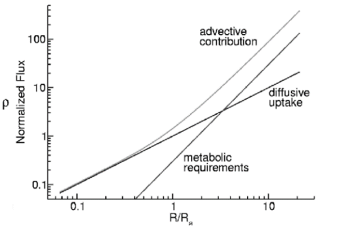
Fig. 6. Graph representing the metabolic fluxes as a function of the colony’s radius. First, fluid advection is the main nutrient supplier to the organism, and its importance rises with the latter’s size. Also, the amount of metabolites received by each cell increases with the number of cells making up the colony, thus making multicellularity advantageous (Goldstein, 2010).

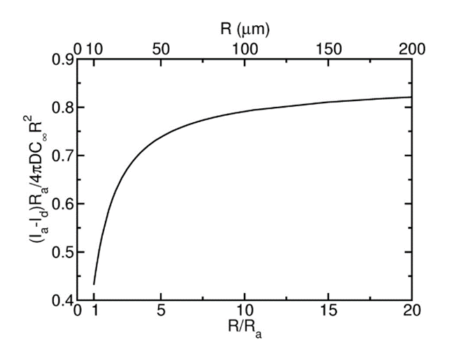
Fig. 7. Difference between molecular flux plotted in function of the colony radius. The advective contribution outweighs nutrient diffusion at R = R_a, and the benefit provided by the latter becomes negligible at 10 R_a, as materialized by the asymptotic behavior of the curve as R reaches infinity.

The role of randomness during self-assembly

During the growth of a juvenile spheroid, somatic cells start assembling together to form an almost perfectly spherical shape. The fact that this complex and functional arrangement is dictated by self-assembly makes it particularly subject to random noise (Zeravcic & Brenner, 2014), which may alter the final structure of the colony. Randomness can manifest itself in a variety of ways, such as variability in cell growth or in the interactions between cells during their assembly. In other words, these unpredictable effects are likely to alter the manner in which somatic cells are packed on the colony’s surface, thus preventing it from being fully functional. This observation leads to the following question: how can unregulated assembly result in a reliable spherical geometry of the colony?

Surprisingly, fluctuations in cell packing geometry have been shown to follow a universal distribution. More specifically, the level of randomness is governed by the maximum entropy principle (Day et al., 2022). In Volvox’s case, this concept relates cellular randomness to the properties of the multicellular organism.

Concretely, it works by enumerating all cellular configurations within the colony. To do so, the latter is considered as a volume V made of N cells, and the overall system can be represented via a Voronoi tessellation. Finally, the maximum entropy principle follows a gamma distribution which describe the most probable distribution of different volumes for the N cells (Aste & Di Matteo, 2008).
Microscope imaging techniques enabled researchers to construct a 2D Voronoi tessellation of somatic cells, as seen in Fig. 8. The level of randomness is characterized by the properties of each cell’s neighborhood, which is represented by the variety of angles between tiles and their respective area. Moreover, comparing this real data with the gamma distribution predictions confirmed that the organization of Volvox colonies follows the maximum entropy principle. In other words, the spherical shape is the most likely to occur in Nature, which is why all colonies adopt it during self-assembly. This shows, just like in the first section, that spherical shapes are ideal. To conclude, while random noise can result in phenotypic variability, it rather helps the species develop robust features and highly predictable patterns that are easily heritable (Day et al., 2022).

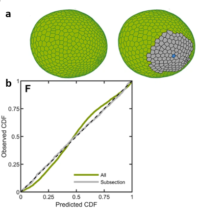
Fig. 8. (a) Voronoi tessellations in two dimensions of the same Volvox colony, with the gray area representing a subsection that was more intensively studied. Each tile corresponds to the space related to a somatic cell, whose variations are materialized by the tile’s shape and size. (b) This graph compares the empirical cumulative distribution to the predicted entropic distributions for the somatic cell properties. The dashed black line represents the hypothetical perfect agreement between experimental data and predictions inferred from the maximum entropy principle.

Although randomness only induces cellular area heterogeneity that has no impact on the colony’s shape, it may affect its motility. However, as several studies have demonstrated, flows around the microalgae are surprisingly smooth. As a matter of fact, the intensity of the flow generated by a given flagellum is inversely proportional to the distance from the flagellum (Boselli et al., 2021). Since this decay is linear and relatively slow, one can infer that the contribution of many flagella makes local fluid flow variations negligible (Day et al., 2022). In other words, flow variations caused by differences in cellular areas have no effect on the organism’s motility since the collective behavior tends to compensate, thus leading to an overall smooth flow.

Modeling the motion of a volvox colony in three dimensions

Volvox’s wonderful dances have always fascinated and attracted researchers. As a result, the stability of several Volvox colonies interacting with each other has been extensively studied, thus almost comprehensively unveiling the collective behavior of the species. Consequently, this preference makes the knowledge of the motion of a single colony still very limited (Elgeti et al., 2015).
Setting fractal dimensions aside, a colony can be considered as a sphere in three dimensions. Since the number of somatic cells making up the sphere surface may vary from 500 to 50 000, the mass M and center of mass $\vec{R}$ of the sphere are subject to change (Herron, 2016). To account for this factor, the center of mass of a colony of N cells with mass $\m_i$ and distance from the center of mass $\vec{r}_i$ is defined as $\vec{R} = \frac{1}{M} \sum_{i=1}^{N} m_i \vec{r}_i$ (Dini et al., 2022) (see Fig. 9).

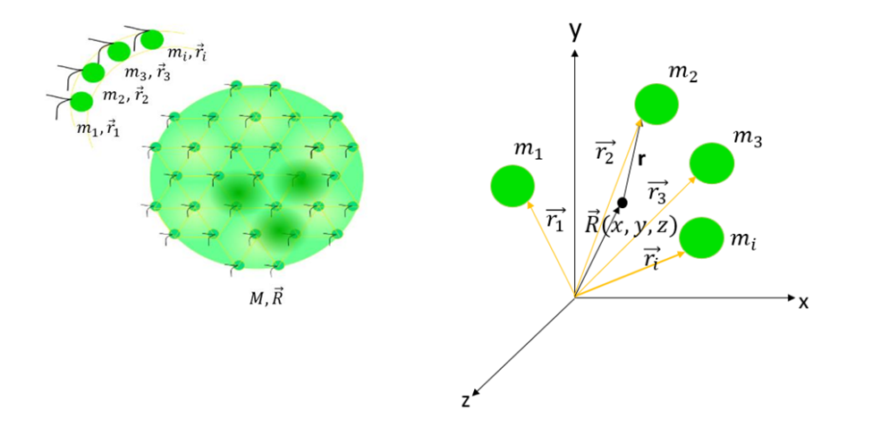
Fig. 9 The left picture is a model of a Volvox colony made of somatic cells. These are characterized individually and have different masses $\m_i$ and distances $\vec{r}_i$ from the center of mass, as shown in the three-dimensional plane on the right.

Owing to the shape of the colony, changing variables from cartesian coordinates to spherical coordinates considerably facilitates further derivations. This framework is defined as follows (Anthonys, 2014), and is illustrated in Fig 10.

$\begin{equation*} \begin{cases} x = r \sin \phi \cos \theta, \\ y = r \sin \phi \sin \theta, \\ z = r \cos \phi. \end{cases} \end{equation*}$

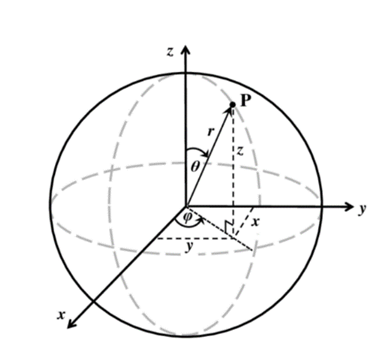
Fig. 10. Illustration of the spherical coordinate system, endowed with a translational parameter $\vec{r}$ and two rotational degrees of freedomφ and θ.

This system is particularly suited to Volvox, as it greatly simplifies the study of rotational movements which are at the core of the colony’s motion. Varying the parameters leads to three equations that describe translational, rolling, and spinning motions. More specifically, the first refers to a change in r, the second to a change in θ, and the last to a change in φ (Dini et al., 2022).
Translation:

$\text{Translation: } \left\{\begin{aligned}x(t) &= x(0) + v_x t, \\y(t) &= y(0) + v_y t, \\z(t) &= z(0) + v_z t.\end{aligned}\right.$

Rolling: $\theta(t) = \theta(0) + \omega_{\theta} t$

Spinning: $\varphi(t) = \varphi(0) + \omega_{\varphi} t$

These series of equations describe the motion of a spherical colony in any direction. It is crucial to note that $\vec{r}$ is a vector, which is decomposed into cartesian coordinates to study translational motion. Also, the linear and angular velocities of the sphere in the ith direction are respectively v_i and ω_i.
Using these equations with varying conditions, it is possible to model the motion of an individual colony in its surroundings by creating algorithms. Moreover, the comparison of the predicted outcomes with real observations determines which parameters yield a realistic model. This model then enables researchers to gain insight into the variations in the mass among several somatic cells for example. Indeed, measuring this property manually to infer conclusions is not feasible given the scale involved. The study performed by Dini et al. in 2022 concluded that the motion of a colony independent from external factors mainly narrows down to translational and spinning mechanisms. Therefore, the combination of mathematical and computational tools will be of paramount importance to complete and confirm all the qualitative data collected so far about Volvox.
Nevertheless, it is important to acknowledge that this model is a simplified version of a colony. As a matter of fact, further improvements could be made by taking into account both the flagella and the germ cells within the spherical shell made of somatic cells to improve the model.

The squirmer model for volvox swimming

Mathematical models prove to be extremely useful when attempting to predict patterns in life. Notably the movement of living organisms. While not perfect, the trends observed often follow well-known equations and can be modelled after careful study. From this, we can also make guesses that movement will follow equations for already determined movement in certain mediums and thus from these equations we can make discoveries. The process of using math can go both ways. A good example of this is the squirmer model for analyzing the swimming of Volvox. Of note, Volvox swims through the use of flagella with an axis of symmetry in the direction of movement. However, it has an approximate 20-degree azimuthal tilt. This causes the rotation of Volvox about a fixed axis as it swims, complicating the modelling of its movement. As well, the colony is tilted upward due to an imbalance of density between the front and back of the colony. Finally, the radius of the colony varies from one group to another adding another variable to the model on top of the fact that this radius will change throughout its lifespan (Pedley et al., 2016).

Relationship between colony size and speed

First, we can make interesting predictions and inferences by comparing the colony sizes with the upstream swimming speed of Volvox. This relation has been modelled and is shown in Fig. 11.. By observing the graphs, we see that as expected, the swimming speed as well as the angular velocity do decrease with an increase in size. This makes sense, because an increased radius will increase drag (as we know from the formula for drag). On top of this, we can agree with the info we are seeing because the sedimentation speed, which is the speed at which the colony sinks, follows a rough linear equation. This makes sense because sedimentation would follow the Stokes equation which would be linear because we have a very low Reynolds number (<0.1). We can see here again that not only can we develop a formula for swimming speed based on colony size, but we can validate it by using our knowledge of known mathematics to check its relation to other things we know to be true (Pedley et al., 2016).

Formula for drag:

$F_D = \frac{1}{2} \rho v^2 C_D A ;$

ρ: density,ν: speed of the object,
C_D: drag coefficient, A: cross sectional Area
Stokes equation example (x-component):

X–momentum = $\text{X-momentum} = - \frac{\partial \rho}{\partial x} + \frac{1}{Re_r} \left[ \frac{\partial \tau_{xx}}{\partial x} + \frac{\partial \tau_{xy}}{\partial y} + \frac{\partial \tau_{xz}}{\partial z} \right]; coordinate: (x,y,z)$

Re: Reynolds number,ρ: density,τ: stress

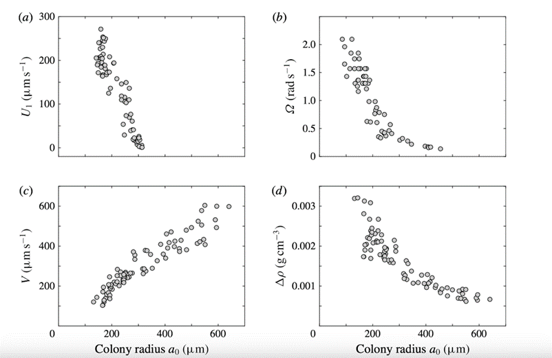
Fig. 11. Swimming properties of Volvox as a function of colony radius a_0. Measured values of the (a) upswimming speed U₁, (b) angular velocity Ω, and (c) sedimentation speed V, as well as (d) the deduced density offset $\Delta \rho = \frac{9 \mu V}{2 g a_0^2}$ compared with the surrounding medium (Pedley et al., 2016).

Mathematical model for velocity

While the observation of the colony size was interesting, we didn’t develop a working formula for modelling movement. Thus, let’s create a preliminary model assuming a zero Reynold’s number and using the Stokes equation for movement in a liquid. Because Volvox rotates as it moves, we will need to include both radial and tangential velocity. Our equations will be expressed as infinite series:

$u_r (r,\theta_0)= - U \cos\theta_0 + A_0 \frac{a^2}{r^2} P_0 + \frac{2}{3}(A_1+B_1)\frac{a^3}{r^3} P_1 + \sum_{n=2}^{\infty} \left[ \left( \frac{1}{2n} \frac{a^n}{r^n} - \frac{1}{2n - 1}\frac{a^{n+2}}{r^{n+2}} \right) A_n P_n + \left( \frac{a^{n+2}}{r^{n+2}} - \frac{a^n}{r^n} \right) B_n P_n \right]$

$u_{\theta} (r,\theta_0) = U \sin\theta_0 + \frac{1}{3}(A_1+B_1)\frac{a^3}{r^3} V_1 + \sum_{n=2}^{\infty} \left[ \left( \frac{1}{2n} \frac{a^{n+2}}{r^{n+2}} - \frac{1}{2n - 1}\frac{a^n}{r^n} \right) B_n V_n + \frac{1}{2n}\left(\frac{1}{2n - 1}\right)\left(\frac{a^n}{r^n} -\frac{a^{n+2}}{r^{n+2}} \right) A_n P_n \right]$

Also, it is important to note that here polar coordinates are used and P_n cos(θ) are Legendre polynomials. V_n can be derived based on a relation with P_n. On top of this, we can also derive the following formula to be used for finding the missing variables when testing (Pedley et al., 2016):

$V_n \cos(\theta) = \frac{2}{n(n+1)} \sin(\theta_0) P_n'(\cos\theta_0)$

Now that we have these formulas for modelling Volvox movement, we can make multiple inferences when comparing to a schematic diagram identified by Blake through analysis of the Volvox colony in Fig. 12..

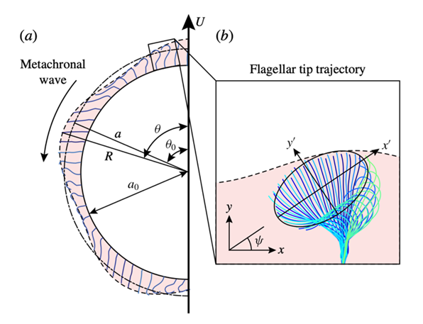
Fig. 12. (a) Schematic diagram of a spherical Volvox colony at one instant in time, with beating flagella and the envelope of flagellar tips. The radius of the extracellular matrix in which the flagella are embedded is a_0. The mean radius of the envelope is a: (R, θ) are the coordinates of a surface element whose average position is (a, θ₀). (b) Measured tip trajectory over multiple beats of a single Volvox flagellum. The trajectory is fitted with an ellipse, which is rotated at an angle 𝜓 with respect to the local colony surface (Pedley et al., 2016).

Defining the variables

This is a perfect example of how we can compare theoretical mathematical models we know to accurately model a certain organism along with data collected from studying that organism to make interesting connections between the two. For example, from 12b we can see that the flagellar beat is approximately elliptical. This elliptical shape appears to have a center at about ⅔ of the total flagellar length. Therefore, we can infer that since we defined a to be the mean radius of the flagella we assume that $a \approx a_0 + \frac{2}{3} L$ , where L is the total flagellar length. We are slowly able to refine our formula through careful inspection and relation between our known mathematical models and data collected from our specific organism Volvox (Pedley et al., 2016).
Now that we have a strong model for predicting the movement of Volvox we just need a few more formulas to define our missing variables and completely refine our formula. These missing variables are A_n, B_n, C_n, and U. Thankfully, these can be derived from the formulas for α_n, β_n, and γ_n which can be defined using the following formulas (where k is the wavenumber, σ is the radian frequency, and χ is the phase difference which are all values that can be determined from physical observations) (Pedley et al., 2016):

$\alpha_0 (t) + \sum_{n=2}^{\infty} \alpha_n (t) P_n (\cos\theta_0) = \sin(k\theta_0 - \sigma t)$

$\sum_{n=1}^{\infty} \beta_n (t) V_n (\cos\theta_0) = \delta \sin(k\theta_0 - \sigma t - \chi)$

$\sum_{n=1}^{\infty} \gamma_n (t) V_n (\cos\theta_0) = \tau \delta \sin(k\theta_0 - \sigma t - \chi)$

Observations using the model for velocity

So far, we have only modelled the velocity components of Volvox so how does this help us determine position? Once again, an interesting and useful property of mathematics arises. Because of derivatives and integrals, we can make relations between things connected by these two relations. Thus, since the integral of velocity would give us position, this formula (if it is integrable) will be able to provide a model for position as well. On top of this, if we were to plug this formula for velocity into online modelling software, we would see that it models a wave function. This is exactly what we would expect from a model being propelled by flagella which are known to produce metachronal waves.
Some of the formulas, derivations, and calculations were omitted to be more concise. However, we can see that from the first two equations mentioned, we have developed a working formula for modelling Volvox movement as well as the ability to correctly define all of our variables. Yet, due to the unpredictability of the living world, this formula is not perfect. The flagellar beating while representing a wave is not perfectly modelled by a sine wave as we have chosen. The simplification is close but not 100% accurate. We assume Volvox to have a perfectly spherically impenetrable membrane which is another oversimplification. Still, this model is a valuable resource as it allows us to simplify the complexity of our living organism and make it easier to do further research on it. Instead of randomly trying to make predictions about Volvox we can now have more accurate starting points.

A mathematical model of volvox embryo inversion

Volvox embryos consist of spherical monolayers, or cells sheets, that need to invert themselves through a process called inversion in order to achieve their adult configuration. This is because they need to have their gonidia on the inside and their somatic cells on the outer surface of the spheroid so that their flagella can extend out of the extracellular matrix to help move the colony around. There are two types of deformation sequences in order to achieve this inversion: type A and type B inversions. These two types of inversion processes have been studied at length, and mathematical models have been developed to describe the motion of the cells during inversion. This section will discuss how these mathematical models were developed. Type B inversion will be discussed first since type A inversion builds on the model used to describe type B inversion (Haas & Goldstein, 2018).

Type B inversion

In the type B inversion sequence, the embryo starts with a circular invagination (folding back on itself) at the equator. The bottom (posterior) hemisphere slowly inverts itself while moving upwards inside of the top (anterior) hemisphere while the phialopore widens. It keeps widening until the inverted bottom hemisphere can pass through the phialopore before the rest of the cell sheet finishes inverting. This process is shown in this short video, which has been accelerated since the actual duration of the inversion takes 45 to 80 minutes (Höhn et al., 2015). It is interesting to study this type of inversion because it shares the process of invagination that is crucial in the process of gastrulation in early animal development (Höhn et al., 2015).
A 2015 study by Höhn et al. used embryos of Volvox globator to develop the first mathematical model of the dynamics of type B inversion in specific stages. This model tests the theory that local changes in intrinsic curvature can in fact drive inversion. The parameters include the thickness h of the elastic spherical cell sheet, which is also referred to as a shell, and the undeformed radius of the shell R under quasistatic variations of its intrinsic curvature. Then, the arclength s along the undeformed shell and the distance r₀ (s) to the axis of revolution, and the corresponding variables S(s) and r(s) for the deformed shell. These quantities are visually represented in Fig. 13.a and b. The meridional stretch f_s is defined as the deformed arclength of a small element over the undeformed arclength of a small element of the shell as follows:

$f_s = \frac{dS}{ds}$

The circumferential stretch $f_{\phi}$ is defined as the ratio of the distance to the axis of revolution of the deformed shell over the undeformed shell (Höhn et al., 2015).
$f_{\phi} = \frac{r}{r_0}$

These stretches are better visualized in Fig. 13.c that shows an enlargement of a small element of the cell sheet. Then, the meridional strain E_s is defined as $E_s = f_s - f_s^0$ , where $f_s^0$ is the preferred stretch of the Helfrich model for membranes and generalizations that have area elasticity (Höhn et al., 2015). The circumferential strain $E_ϕ$ is defined as $E_{\phi} = f_{\phi} - f_{\phi}^0$ , where once again $f_ϕ^0$ is the preferred stretch. The meridional curvature strain Κ_s is defined as $\kappa_s = f_s \kappa_s - f_s^0 \kappa_s^0$ , where κ_s is the meridional curvature of the deformed shell and $κ_s^0$ is its preferred value under the Helfrich model. The circumferential curvature strain Κ_ϕ is defined as $\kappa_{\phi} = f_{\phi} \kappa_{\phi} - f_{\phi}^0 \kappa_{\phi}^0$ , where κ_ϕ is the circumferential curvature of the deformed shell and $\kappa_{\phi}^{0}$ is the corresponding preferred value (Höhn et al., 2015).

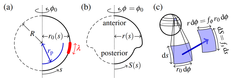
Fig. 13. Visualization of the Elastic Model for Type B embryo inversion. (a) The undeformed elastic spherical shell of radius R and thickness h, showing the arclength s and the distance from the axis of revolution r₀. (b) The deformed configuration of the spherical shell showing the corresponding parameters. (c) Enlargement of a small element of the shell showing undeformed and deformed geometries, which are related by the stretches $f_s$ and f_ϕ.
The study then used a Hookean model to describe the energy of the deformed shell with elastic modulus E and Poisson ratio ν (Höhn et al., 2015). The deformed shell therefore minimizes the energy ℇ as follows:

$\epsilon = \frac{\pi E h}{(1-\nu^2)} \int_0^{\pi R} r^0 (E_s^2 + E_{\phi}^2 + 2\nu E_s E_{\phi}) \, ds + \frac{\pi E h^3}{12(1-\nu^2)} \int_0^{\pi R} r_0 (\kappa_s^2 + \kappa_{\phi}^2 + 2\nu \kappa_s \kappa_{\phi}) \, ds$

This model was used to test whether the initial invagination that occurs at the equator and the movement of the bottom hemisphere are in fact driven by local changes in intrinsic curvature (Höhn et al., 2015). A region of width λ forming below the equator (shown in Fig. 13.a) was considered with preferred curvature $\kappa_{s}^{0} = -k < 0$ and the examination of thin sections showed a value of λ≈0.1πR and kR≈ 10-20. It was found that solely fixing the preferred curvature results in a “purse-string” effect over large ranges of k and λ, which is shown in Fig. 15.a. However, this is not the case in Volvox globator embryos, which have a mushroom shape at this stage. This suggests that cell shape changes are also needed to drive this inversion process (Höhn et al., 2015). To account for this factor, a reduced posterior radius r_p was defined, where r_p < R, and the preferred values for strain and curvature strain were adjusted. More realistic values were found to be $\frac{r_p}{R} < 7$ and kR = 20, and the modified model now yielded mushroom shapes. The modified preferred values for $f_s^0, \quad f_{\phi}^0, \quad \kappa_s^0, \quad \text{and} \quad \kappa_{\phi}^0$ are shown in Fig. 14. (Höhn et al., 2015).

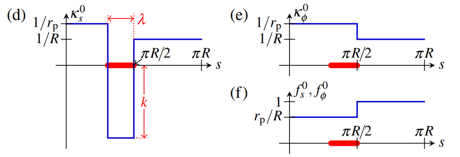
Fig. 14. Imposed intrinsic curvature $\kappa_{s}^{0} = -k < 0$ in a region of width λ along the shell, just below the equator, with modified intrinsic properties due to the new parameter of the posterior radius $r_p<R$ (Höhn et al., 2015).

During inversion of Volvox globator embryos, cells in the bend region change shapes to become more wedge shaped as invagination begins, and more become wedge shaped as it progresses. This is accounted for in the model by using larger values of k and λ, and this allows the contracted posterior to invert inside the anterior hemisphere (Höhn et al., 2015). This is illustrated in Fig. 15..

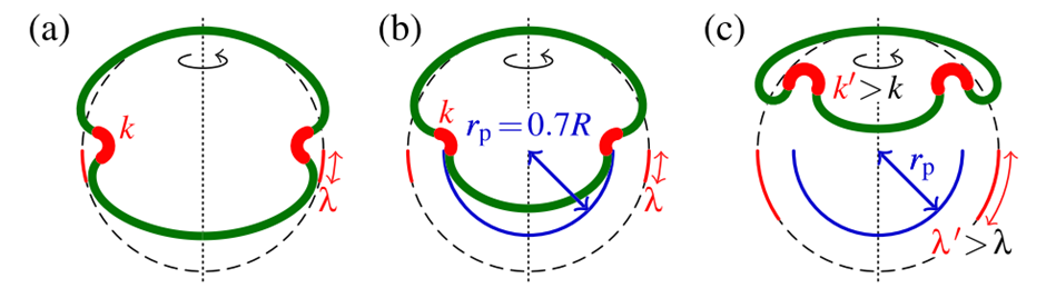
Fig. 15. Results of the elastic model. (a) When the posterior hemisphere is not contracted, there is a “purse-string” effect. (b) The correct mushroom shapes are achieved once posterior contraction is included (due to cell shape changes). (c) This allows the inverted posterior hemisphere to fit inside the anterior hemisphere (Höhn et al., 2015).

It is important to note that defining an expanded anterior radius would achieve the same effect as the defined reduced posterior radius as both would allow the formation of mushroom shapes. It seems that in vivo, both of these take place (Höhn et al., 2015). Unlike Volvox globator, Volvox aureus (another species that undergoes type B inversion) adopts an hourglass shape as show in Fig. 15.a before changing to a mushroom shape, which suggests that the beginning of inversion is only driven by changes in intrinsic curvature in V. aureus, with active contraction and expansion taking place later. As a result, it can be deduced that contraction of the posterior hemisphere and the expansion of the anterior hemisphere are used together to induce mushroom shapes but the timing changes according to the species (Höhn et al., 2015).
Overall, the simple mathematical model shows that Volvox combine changes in intrinsic curvature along with active contraction and expansion to achieve type B inversion. These driving forces allow this amazing green alga to overcome the geometric constraints that would normally make it impossible to turn a spherical cell sheet inside out to achieve embryo inversion (Höhn et al., 2015).

Type A inversion

In type A embryonic inversion, which occurs in Volvox carteri, four lips open up at the phialopore of the spherical cell sheet and peel back to achieve inversion. The phialopore is a cross-shaped opening at the anterior pole, the only spot in the spherical cell sheet where the cells are not connected by cytoplasmic bridges, which are thin tubes that result from incomplete cell division (Haas & Goldstein, 2018). The different steps of this inversion sequence are shown in Fig. 16..

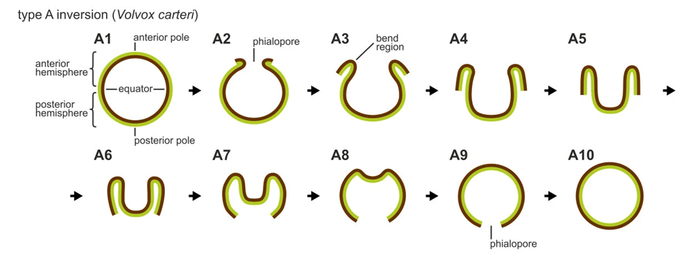
Fig. 16. Simplified schematic representation of type A inversion in Volvox carteri (Höhn & Hallmann, 2011).

A 2018 study by Haas & Goldstein analyzed the mechanics of the opening of the phialopore by the peeling back of the four lips and derived an averaged elastic model for the lips in Volvox carteri. The same initial parameters as in type B inversion will be used for type A, including radius R, thickness h, arclength s, distance from the axis of revolution $r_0$ , as well as meridional and circumferential stretches $f_s$ and $f_ϕ$ . Then, the shell is divided into N lips of angular extent (maximum angle) $2\phi = \frac{2\pi}{N}$ , which is shown in Fig. 17.b. The azimuthal angle ϕ of the undeformed sphere or shell is also shown in Fig. 17.a and b. The azimuthal angle ϕ ̅ of the deformed shell is restricted to uniform stretching or compression and is defined as ϕ ̅=Φ(s)ϕ (Haas & Goldstein, 2018).

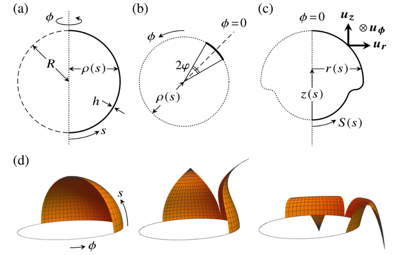
Fig. 17. Representation of the elastic model for type A embryo inversion. (a) The undeformed shell geometry. (b) Anterior view of the lips showing a cut in a plane containing the axis of symmetry which define N lips with an angle extent -φ≤ϕ≤φ. (c) The deformed shell geometry at the midplane ϕ=0 of the lip showing a local basis $(u_r, u_{\phi}, u_z)$ . (d) The deformation of two lips according to the geometric simplification (Haas & Goldstein, 2018).

Now, considering a right-handed set of coordinate axes $(u_r, u_{\phi}, u_z)$ as shown in Fig. 17.c, the position vector of a point on the mid-surface of the deformed shell can be defined as:

$\mathbf{r}(s,\phi) = r(s) \mathbf{u}_r (\Phi(s)\phi) + z(s)\mathbf{u}_z$

The meridional and circumferential tangent vectors to the deformed mid-surface can be defined as (Haas & Goldstein, 2018):

$e_s = r' u_r + r \Phi' \phi u_{\phi} + z' u_z$
$e_{\phi} = r \Phi u_{\phi}$

Where the prime notation is used to denote differentiation with respect to arclength s (Haas & Goldstein, 2018). By definition, $(r')^2 + (z')^2 = f_s^2$ so $r' = f_s \cos\beta$ and $z' = f_s \sin\beta$ . The metric of the mid-surface can be written as:

$\left( f_s^2 + r^2 (\Phi')^2 \phi^2 \right) \, ds^2 + r^2 \Phi^2 \, d\phi^2 + 2 r^2 \Phi \Phi' \phi \, ds \, d\phi$

The second fundamental form of this equation (Haas & Goldstein, 2018) is:

$\left( f_s \beta' + r (\Phi')^2 \phi^2 \sin\beta \right) ds^2 + r \Phi^2 \sin\beta d\phi^2 + 2 r \Phi \Phi' \phi \sin\beta \phi ds d\phi$

The unit normal vector to the mid-surface of the deformed shell (Haas & Goldstein, 2018) is:

$\mathbf{n} = \cos\beta \mathbf{u}_z - \sin\beta \mathbf{u}_r$

Then, the Weingarten equations (Haas & Goldstein, 2018) give:

$\frac{\partial \mathbf{n}}{\partial s} = -\kappa_s \mathbf{e}s + \frac{\Phi' \phi}{\Phi} (\kappa_s - \kappa{\phi}) \mathbf{e}_{\phi}$
$\frac{\partial \mathbf{n}}{\partial \phi} = -\kappa_{\phi} \mathbf{e}_{\phi}$

Where $\kappa_s = \frac{\beta'}{f_s}$ and $\kappa_{\phi} = \frac{\sin\beta}{r}$ are the main curvatures of the midline of the lip (Haas & Goldstein, 2018).

Then, the elastic strains were calculated. The Kirchhoff hypothesis, which states that the normal vectors to undeformed shell mid-surface remain normal to the deformed shell mid-surface, was used to calculate the deformation gradient F^g. The intrinsic deformation gradient tensor F⁰ was also defined (Haas & Goldstein, 2018). Then, taking a coordinate ζ across the thickness of the shell, the meridional and circumferential strains (Haas & Goldstein, 2018) were approximated as follows:

$f_s (1 - \kappa_s \zeta) \approx f_s^0 (1 - \kappa_s^0 \xi)$

$f_{\phi} (1 - \kappa_{\phi} \zeta) \approx \frac{f_{\phi}^0 (1 - \kappa_{\phi}^0 \xi)}{\Phi}$

Finally, the elastic energy was derived using the assumption that the shell is made of a Hookean material, as in type B inversion, and has an elastic modulus E and a Poisson’s ratio υ. Then, the elastic energy (Haas & Goldstein, 2018) is:

$\frac{\mathcal{E}}{2\pi r_0} = \frac{E}{2(1-\nu^2)} \int_{-h/2}^{h/2} \left[ (\varepsilon_{ss} + \varepsilon_{\phi\phi})^2 - 2(\nu-1)(\varepsilon_{ss} \varepsilon_{\phi\phi} - \varepsilon_{s\phi} \varepsilon_{\phi s}) \right] d\phi \, d\zeta$

The integrals were then solved numerically with respect to ϕ and ζ using the boundary-value problem solver bvp4c of MATLAB (Haas & Goldstein, 2018).

In order to describe the geometry of the undeformed shell, the number of lips N was chosen as N=4, the relative thickness h/R of the cell sheet was chosen as $\frac{h}{R} = 0.21$ , the opening angle P of the phialopore was chosen as P=0.3, and the extent of the lips l was chosen as l=0.7 (Haas & Goldstein, 2018). Then, the value of the curvature of the flask cells was set as k=κ_flask and the posterior limit of the bend region is set at θ=Θ. Starting from the undeformed shell, the bend region was propagated from the tip of the lips to their base and then to the posterior pole by decreasing the value of Θ (Haas & Goldstein, 2018). This leads to two types of behavior separated by a critical value k_*, where if k>k_*, then the shell inverts on the path of lowest energy, and if k<k_*, then the shell does not invert on the path of lowest energy. The flip-over behavior of the lips is shown in Fig. 18. (Haas & Goldstein, 2018). As the value of k=κ_flask decreases towards the critical value k, the lips open wider and wider before flipping over and the opening of the phialopore decreases very fast after this flip-over. However, as =κ_flask falls below the critical value k_*, the maximum radius of the phialopore decreases and the lips do not flip over (the phialopore just widens and remains open) (Haas & Goldstein, 2018). Fig. 18. The flip-over of the lips. The radius of the phialopore r_phial normalized against its initial value is plotted against the posterior limit angle of the bend region Φ on the path of lowest energy for different values of k=κ_flask (Haas & Goldstein, 2018).

Fig. 18. The flip-over of the lips. The radius of the phialopore r_phial normalized against its initial value is plotted against the posterior limit angle of the bend region Φ on the path of lowest energy for different values of $k = \kappa_{\text{flask}}$ (Haas & Goldstein, 2018).

One important conclusion in this study is that contrary to type B inversion, which was discussed earlier, type A inversion in Volvox carteri mechanically does not require contraction and expansion of the posterior and anterior hemispheres of the cell sheet. In fact, due to the presence of peeling lips, the inversion is facilitated and does not rely on active contraction and expansion (Haas & Goldstein, 2018).

Conclusion

Volvox have yet again managed to amaze us through their amazing properties. They have shown to us through analysis of their fractal dimension that they can be a complex organism relative to unicellular or colonial green algae even while visually demonstrating simple shapes and patterns. They have also shown us how large of a gap there really is between a simple multicellular organism and its colonial/unicellular ancestors, at least in terms of morphology of the organisms as a whole. This of course, does not happen easily, and measures must be taken to adapt to this multicellular body.
In fact, according to biological laws, Volvox colonies are too large for the passive diffusion of metabolites to meet their needs. Therefore, the species takes advantage of the fluid flow generated by flagella for the colony’s motion, which induces the phenomenon of fluid advection. Concretely, these external forces drive particles present in the surroundings towards Volvox, which increases the number of metabolites received per somatic cell. Hence, the more somatic cells, the higher the importance of fluid advection, and the more benefits for each cell! In other words, Volvox turned the potential issue related to multicellularity into an advantage.
Furthermore, Volvox adopted a spherical shape, which naturally occurs during the growth and organization of a juvenile colony. This shape has been shown to have the lowest fractal dimension among the shapes presented by most green algae, implying a simple and more ideal form. The natural adoption of this form therefore further facilitated the transition to multicellularity.
One design solution that can be observed from the squirmer model we derived is that a low Reynolds number is beneficial for movement of Volvox. Not only does it reduce external forces and simplify the mathematical model for swimming, but it also reduces drag. The reduced drag will make swimming easier. So, from our observation, we see Volvox can ensure it is most often in a low Reynolds number medium allowing it to have an easier lifestyle.
Finally, Volvox have found a way to achieve what seems incredibly difficult: turning the spheroid monolayer or cell sheet of its embryo inside out. This paper discussed the mathematical models that were developed to describe this process. The main takeaways from type B inversion are that this was only possible due to active contraction of the cells in the posterior hemisphere and expansion of the cells in the anterior hemisphere, as well as propagating changes in intrinsic curvature. As for type A inversion, the mathematical model for the peeling of the lips explained how they make this process possible.
This paper once and for all demonstrates that Volvox have mastered the transition to multicellularity and have optimized their morphology and behavior to be able to survive and overcome all obstacles that could possibly come in their way.

References

3Blue1Brown. (2017, Jan 27). Fractals are typically not self-similar [Video]. Youtube. https://www.youtube.com/watch?app=desktop&v=gB9n2gHsHN4&ab_channel=3Blue1Brown

Anthonys, G. (2014). Application of translational addition theorems to the study of the magnetization of systems of ferromagnetic spheres.

Aste, T., & Di Matteo, T. (2008). Emergence of Gamma distributions in granular materials and packing models. Physical Review E, 77(2), 021309.

Boselli, F., Jullien, J., Lauga, E., & Goldstein, R. E. (2021). Fluid mechanics of mosaic ciliated tissues. Physical review letters, 127(19), 198102.

Day, T. C., Höhn, S. S., Zamani-Dahaj, S. A., Yanni, D., Burnetti, A., Pentz, J., Honerkamp-Smith, A. R., Wioland, H., Sleath, H. R., & Ratcliff, W. C. (2022). Cellular organization in lab-evolved and extant multicellular species obeys a maximum entropy law. Elife, 11, e72707.

Dini, S. U., Nurafni, S., Fairuza, A. Z., & Taufik, I. (2022). Modelling of Motion of a Volvox Colony using Many-Body System and Its Qualitative Comparison with Observations. Journal of Physics: Conference Series,

Elgeti, J., Winkler, R. G., & Gompper, G. (2015). Physics of microswimmers—single particle motion and collective behavior: a review. Reports on progress in physics, 78(5), 056601.

Goldstein, R. E. (2010). Evolution of biological complexity. Biological Physics: Poincaré Seminar 2009,

Haas, P. A., & Goldstein, R. E. (2018). Embryonic inversion in Volvox carteri: The flipping and peeling of elastic lips. Physical Review, 98(5). https://doi.org/10.1103/physreve.98.052415

Herron, M. D. (2016). Origins of multicellular complexity: Volvox and the volvocine algae. In: Wiley Online Library.

Höhn, S., & Hallmann, A. (2011). There is more than one way to turn a spherical cellular monolayer inside out: type B embryo inversion in Volvox globator. BMC Biology, 9(1). https://doi.org/10.1186/1741-7007-9-89 ‌

Höhn, S., Honerkamp-Smith, A. R., Haas, P. A., Trong, P. K., & Goldstein, R. E.. (2015). Dynamics of a Volvox Embryo Turning Itself Inside Out. Physical Review Letters, 114(17). https://doi.org/10.1103/physrevlett.114.178101

Kenkel, N. C., & Walker, D. J. (1996). Fractals in the Biological Sciences. Coenoses, 11(2), 77-100.

Kirk, D. L., Birchem, R., & King, N. (1986). The Extracellular Matrix of Volvox: A Comparative Study and Proposed System of Nomenclature. Journal of Cell Science, 80(1), 207-231. https://doi.org/10.1242/jcs.80.1.207

Koehn, D., Piazolo, S., Beaudoin, N. E., Kelka, U., Spruženiece, L., Putnis, C. V., & Toussaint, R. (2021). Relative rates of fluid advection, elemental diffusion and replacement govern reaction front patterns. Earth and Planetary Science Letters, 565, 116950.

Niklas, K. J. (2000). The evolution of plant body plans—a biomechanical perspective. Annals of Botany, 85(4), 411-438.

Pedley, T. J., Brumley, D. R., & Goldstein, R. E. (2016). Squirmers with swirl: A model for Volvox swimming. Journal of Fluid Mechanics, 798, 165–186. https://doi.org/10.1017/jfm.2016.306

Pham, D. T., & Musielak, Z. E. (2023). Spectra of Reduced Fractals and Their Applications in Biology. Fractal and Fractional, 7(1). https://doi.org/10.3390/fractalfract7010028

Short, M. B., Solari, C. A., Ganguly, S., Powers, T. R., Kessler, J. O., & Goldstein, R. E. (2006). Flows driven by flagella of multicellular organisms enhance long-range molecular transport. Proceedings of the National Academy of Sciences, 103(22), 8315-8319.

Solari, C. A., Kessler, J. O., & Michod, R. E. (2006). A hydrodynamics approach to the evolution of multicellularity: flagellar motility and germ-soma differentiation in volvocalean green algae. The American Naturalist, 167(4), 537-554.

Umen, J. G. (2020). Volvox and volvocine green algae. EvoDevo, 11(1), 13. https://doi.org/10.1186/s13227-020-00158-7

Umen, J., & Herron, M. D. (2021). Green Algal Models for Multicellularity. Annual Review of Genetics, 55(1), 603–632. https://doi.org/10.1146/annurev-genet-032321-091533

Zeravcic, Z., & Brenner, M. P. (2014). Self-replicating colloidal clusters. Proceedings of the National Academy of Sciences, 111(5), 1748-1753.