Mathematical Modelling of Dinoflagellate Swimming, Population Dynamics and Interactions with Other Organisms
Thalia Azadian, Arda Barlas, Sophia Chen, Simon Girard
Abstract
Mathematical models have been made to determine the vertical migration of dinoflagellates while considering the availability of nitrogen. Studies have shown that low nitrogen abundances lead to dinoflagellates avoiding sunlight, and not performing diel vertical migration. Dinoflagellate blooms take place under specific conditions of irradiance, temperature, and salinity. A model of the germination dynamics of Dinoflagellate Cysts can be studied in the Alexandrium fundyense species. At a larger scale, the quantitative relationship between the rate of growth of dinoflagellates and the effect of these constraints is examined in the cochlodinium polykrikoides Margalef species. Finally, population dynamics between dinoflagellates and parasites from the genus Amoebophrya that infect them can be modelled using differential equations. Amoebophrya has been identified as a source of population control for blooming toxic dinoflagellates.
Introduction
Dinoflagellates are unicellular protists that live in both freshwater and saltwater systems. In this paper, dinoflagellates will be studied through the lens of mathematics. Mathematics is everywhere in nature. Geometries, rates of change, patterns, and movements of organisms and ecosystems can be described using mathematical techniques. In the following paper, we will discuss the modelling of dinoflagellates’ population dynamics.
Dinoflagellates are responsible for a phenomenon called the Red Tide. Indeed, as dinoflagellate populations bloom at exponential rates, a reddish colour appears in the water as a result of the sheer volume of this microorganism in the ocean. This bloom can have drastic effects on the ecosystem as dinoflagellate toxins lead to the death of many organisms.
In this paper, dinoflagellates populations will be studied using mathematics in four different contexts: their vertical migration, their germination phase, their population growth, and their interactions with parasites from the genus Amoebophrya that frequently infect them (Figure 1).
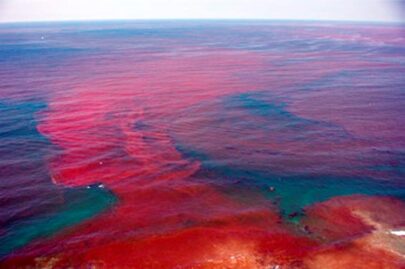
Figure 1: (A) Red tide phenomenon in San Diego, California in 2001 (Zheng & Klemas, 2018).
Vertical migration modelling of dinoflagellates in response to carbon/nitrogen requirements and photosynthesis requirements
Dinoflagellates require multiple sources of nutrients. Ji. et al present a simplified mathematical model of the different needs of dinoflagellates (Ji & Franks, 2007). Dinoflagellates require sunlight and various sources of nutrients such as carbon for energy and nitrogen for amino acids (Ji & Franks, 2007). The authors present a mathematical model that describes the way in which dinoflagellates migrate vertically to optimise their requirements for the best chances of survival.
Dinoflagellates require carbon and nitrogen. Dinoflagellates’ uptake for carbon can be modelled with the differential equation dC/dt = (µ – λ)C, where µ is the growth of the dinoflagellate and λ is the carbon that is removed from the dinoflagellate through respiration (Ji & Franks, 2007). The nitrogen requirements depend is dependent on the amount of carbon that the dinoflagellate has, dN/dt = VC, where V is the amount of nitrogen required per carbon (Ji & Franks, 2007). The ratio of carbon to nitrogen indicates whether an organism has enough nutrients (Cullen & Horrigan, 1981). An issue that dinoflagellates need to solve is to balance photosynthesis for energy and amount of nitrogen. This is because the location where the most nutrients are present is often not the location where sunlight is the most optimal for photosynthesis (Cullen & Horrigan, 1981; Ji & Franks, 2007). The nitrogen quota, Q, is the ratio of nitrogen to carbon that the dinoflagellate requires, which can be modelled as dQ/dt = –(µ – λ)Q + V . Therefore, dinoflagellates are often observed to migrate to get all the resources that they require.
There are multiple patterns in which dinoflagellates migrate in response to their different needs. Diel vertical migration is when dinoflagellates move closer to the surface during the day to receive sunlight for photosynthesis, and asynchronous vertical migration is when dinoflagellates migrate vertically with a period of longer than a day (Ji & Franks, 2007). Dinoflagellates can choose to either follow diel vertical migration or asynchronous vertical migration depending on its needs. Ji and Franks (2007) modelled the time ratio that the dinoflagellates spend in both light and dark environments τlight and τdark:
τ_{dark}=-(V_m/ΔQ-λ)^{-1} * ln[(V_m/(V_m-λΔQ)-γ)/(V_m/(V_m-λΔQ)-(Q_{min}/Q_{max}) σ)]τ_{light}=-(μ_max-λ)^{-1} * ln[(σ-μ_{max}/(μ_{max}-λ))/(Q_{max}/(Q_{min} γ-μ_{max}/(μ_{max}-λ)))]Vm is the maximum uptake of nitrogen, γ is the threshold coefficient for ascent such that Q > γQmax and σ is the threshold coefficient for descent such that Q < σQmin. In experiments, dinoflagellates follow diel vertical migration patterns (Cullen & Horrigan, 1981), which suggests that τlight ≈ 0.5.
Experimentally, the concentration of carbon to nitrogen plays a role in when the dinoflagellate surfaces. When the carbon-to-nitrogen ratio is low (abundant nitrogen), dinoflagellates have a higher capacity for photosynthesis, while a high carbon-to-nitrogen ratio is associated with a lower capacity for photosynthesis (Cullen & Horrigan, 1981). In fact, Cullen and Horrigan (1981) also mention how Heaney and Eppley (1981) found that when nitrogen is depleted, dinoflagellates tend to stay deeper in the ocean and avoid the surface for photosynthesis. However, when nitrogen was added to the pond, dinoflagellates resumed their diel vertical migration patterns, which indicates that when dinoflagellates have an abundance of nutrients, they can take advantage of it and perform photosynthesis for more energy. However, when dinoflagellates lack nitrogen, there is no point for them to surface for photosynthesis, as they cannot take advantage of the energy to perform protein synthesis, and the risk of phototoxicity outweighs the non-existent benefits. Therefore, to conserve energy, the dinoflagellate does not surface, as it also expends energy to counteract gravity when surfacing.
Modeling the germination dynamics of dinoflagellate cysts in harmful algal blooms: a case study on Alexandrium fundyense
Harmful algal blooms (HABs), caused by a variety of dinoflagellate species, pose significant ecological and economic threats. These species, including Alexandrium spp., Pyrodinium bahamense, Gymnodinium catenatum, Cocchlodinium polykrikoides, Pfiesteria piscicida, Chattonella spp., and Heterosigma akashiwo, have a dormant cyst stage crucial for their survival and proliferation. These cysts, found within bottom sediments, act as seedbeds during unfavorable conditions and play a pivotal role in the initiation and decline of HABs (Matsuoka and Fukuyo, 2003).
The dormancy of these cysts is governed by both internal mechanisms, such as mandatory maturation periods post-encystment and an endogenous annual clock observed in Alexandrium fundyense (Anderson and Keafer, 1987; Matrai et al., 2005), and external factors like temperature, light, and oxygen availability (Anderson et al., 1987; Dale, 1983).
Oxygen is particularly crucial for cyst germination. Most dinoflagellate species need oxygen to germinate, and cysts buried deep in sediments either remain dormant or germinate when exposed to oxygenated conditions (Rengefors and Anderson, 1998; Kremp and Anderson, 2000). A. tamarense cysts, for instance, can survive in anoxic sediments for around 5 years, demonstrating the resilience of these organisms (Keafer et al., 1992).
Germination leads to the proliferation of cells in the water column, initiating blooms. These blooms often end with sexual reproduction, occurring when nutrient limitations arise. The zygotes formed then settle and become dormant cysts, completing the life cycle (Anderson and Lindquist, 1985; Pfiester and Anderson, 1987). Despite the crucial role of cysts in HAB dynamics, quantifying their impact, particularly in Alexandrium blooms, is challenging due to the dynamic nature of coastal waters and the logistical difficulties of direct measurement.
In this section, we describe the mathematical modeling of cell flux from germinated cysts within dinoflagellate populations, focusing particularly on Alexandrium fundyense. We explore attempts made during the Ecology and Oceanography of Harmful Algal Blooms (ECOHAB)-Gulf of Maine (GOM) project to estimate the flux of germinated cells indirectly. This involved a combination of laboratory experiments, field measurements, cyst abundance mapping, and numerical modeling to better understand the dynamics of cyst germination and subsequent bloom initiation. Through this approach, we aim to shed light on the complex interplay of environmental cues, cyst dynamics, and bloom formation in these critical HAB species.
Cyst mapping and preliminary studies
In October 1997, a large-scale cyst mapping survey was conducted aboard the R.V. Endeavor across the Gulf of Maine, collecting sediment samples from 79 stations (Anderson et al., 2003). The timing was chosen to ensure that mature cysts were collected after formation but before germination. The survey was expanded in subsequent years to gain more detailed data in specific regions. The hydraulically damped corer was utilized for sample collection, ensuring undisturbed samples for accurate enumeration (Craib, 1965).
The top three centimeters of sediment were processed to separate the cysts, which were then identified and counted using primulin-stained Sedgewick Rafter slides under epifluorescence microscopy (Yamaguchi et al., 1995). This effort, combined with data from additional surveys, provided a comprehensive map of cyst distribution necessary for modeling germination dynamics (White and Lewis, 1982; Martin and Wildish, 1994; J. Martin, unpublished data).
Field studies on cyst fluorescence
Field studies to assess cyst fluorescence were conducted alongside the mapping efforts. Cores taken near Casco Bay were examined for fluorescence to gauge cyst viability and readiness for germination. These studies were careful to only consider the top centimeter of sediment to prevent contamination from lower layers (Anderson et al., 1982).
Laboratory experiments on germination and fluorescence
Laboratory experiments were set up to reflect the environmental conditions of the Gulf of Maine, examining the effects of temperature and light on cyst germination and autofluorescence. Consistency across experiments was maintained to ensure comparability (Guillard and Ryther, 1962; Matrai et al., 2005). Germination potential was assessed for each sediment sample, and incubations were managed to simulate natural conditions as closely as possible (Anderson et al., 2003).
The mathematical model of cell flux from germinated cysts
The mathematical modeling of germination rates involves several environmental and biological factors. The rate of germination (G, % of initial cysts day-1) is influenced by bottom water temperature (T, ℃), irradiance (E, Wm-2), and an endogenous clock (EC(t)) where t is the year-day. The general form of the model is as follows:
G(T,E,t)=EC(t)×G(T,E)
This equation indicates that germination is a function of both temperature and light, and it is further modulated by the organism’s intrinsic biological clock (Anderson & Keafer, 1987; Matrai et al., 2005). For temperature and light dependence, the model uses empirical data to associate a germination rate with specific experimental conditions (Bewley & Black, 1982). It fits a line to the data points, adjusting for the asymptotic nature of germination potential, captured by the following equation:
G(T,E_{lgt} )=G_{min}(E_{lgt} ) +((G_{max}(E_{lgt} ) -G_{min}(E_{lgt} ) )/2)×tanh(α(E_{lgt} )T-β(E_{lgt} ))+1G(T,E_{drk} )=G_{min} (E_{drk})+((G_{max} (E_{drk} )-G_{min} (E_{drk})/2)×[ tanh(α(E_{drk})T-β(E_{drk})+1]The model only considers data prior to 90% germination and within 75 days from the start of experiments to capture the most significant slope that represents the period when most cysts germinate (Anderson, 1998). The fitting process avoids forcing lines through the origin, accounting for any acclimation period required after the cysts are moved from cold, dark storage to experimental conditions (Stock et al., 2005). Although germination rates under laboratory conditions were estimated, they were not used in the germination model.
The model interpolates and extrapolates discrete germination rates to different temperatures using a hyperbolic tangent function, allowing for a linear relationship at moderate temperatures with the slope represented by the variable α (Bewley & Black, 1982). It also accommodates maximum (Gmax) and minimum (Gmin) germination rates over broad temperature ranges, as indicated in the previous equation (Anderson, 1998).
The response to light is modeled similarly, using the following equations to interpolate and extrapolate germination rates based on irradiance values from ‘light’ and ‘dark’ experimental conditions:
G(T,E) = G(T,E_{drk}) + (G(T,E_{lgt})-G(T,E_{drk}))×(E-E_{drk} /(E_{lgt}-E_{drk} )),~E_{lgt}>E>E_{drk}For the purpose of modeling, Edrk (dark conditions) is taken to be 1% of Elgt (light conditions). Sensitivity analyses have shown that this parameter choice does not significantly affect the model’s outcomes (Stock et al., 2005). The attenuation of light reaching the cysts within the sediment is modeled by exponentially attenuating observed surface shortwave irradiance in the water column and within the sediment, with specific attenuation coefficients.
The endogenous clock function (EC(t)) is derived from data across several studies and years, focusing on the first year after cyst isolation to minimize the impact of shifts in the endogenous cycle. Germination potential data is binned by month, and the median of each bin is used to form a representative endogenous clock, with the piecewise function connecting these points.
Finally, the germination function is applied to a cyst map to estimate the cyst flux (Fg) from the sediment, which is formulated as:
F_g=∫_0^1G(T ,E(z),t) × [Cysts cm^{-3} ]_0 dzwhere [Cysts cm-3]0 is the initial number of cysts in the top centimeter of the sediment (Anderson & Keafer, 1987; Matrai et al., 2005). This mathematical model is a complex integration of empirical data, biological rhythms, and environmental parameters to predict the germination rates of cysts in a given habitat.
Implications of temperature salinity and irradiance on the growth rate of Cochlodinium Polykrkoides margalef
Dinoflagellates reproduce both asexually and sexually (U.S. National Office for Harmful Algal Blooms ([National HAB Office], n.d.). Dinoflagellates begin as dormant cysts on the ocean floor (National HAB Office, n.d.). For years, they lay there, waiting for encouraging environmental conditions such as oxygen, temperature, salinity, and irradiance (National HAB Office, n.d.). When the wait is over, the cyst germinates (National HAB Office, n.d.). It cracks open letting out a swimming dinoflagellate (National HAB Office, n.d.). This dinoflagellate begins to reproduce by asexual fission with each new cell dividing into two more (National HAB Office, n.d.). As long as these conditions are present, the dinoflagellate population grows at an alarming rate in a very short amount of time, leading to the red tide phenomena (National HAB Office, n.d.). Once resources are depleted, dinoflagellates begin sexual reproduction with cells developing gametes (National HAB Office, n.d.). A zygotic cell named planozygote is produced as two gametes come together (National HAB Office, n.d.). In turn, the planozygote turns into a cyst by condensing its cell wall and cytoplasm and sinks to the bottom of the ocean, restarting the cycle of the creature (National HAB Office, n.d.).
Hence, the growth rate of this microorganism changes in accordance with these conditions. In section 2, we see the effect of oxygen, temperature, and light when it comes to germination. Now, we will see a similar mathematical analysis on a bigger scale: the complete growth rate of red tide dinoflagellate in relation to temperature, salinity, and irradiance (Kim et al., 2004). The Cochlodinium polykrikoides Margalef dinoflagellate will be used as a model.
Impact of irradiance
Many dinoflagellate species, including the Cochlodinium polykrikoides Margalef, undergo photosynthesis. Hence, the quantity of solar irradiance a dinoflagellate is exposed to has an influence on its growth rate. The mathematical representation of this relation is the following:
μ=μ_m (I- I_0)/((K_S-I_0 )+(I-I_0 ) )
μ=μ_m (I- I_0)/(I+(K_S-2I_0 ) )
where μ is the specific growth rate, μm the maximum specific growth rate, I the irradiance, I0 the compensation irradiance, and Ks the half-saturation irradiance i.e., the irradiance at half of the maximum specific growth rate (μm/2). The compensation irradiance corresponds to the value of irradiance where the rate of photosynthesis matches the rate of cellular respiration.
It was found that the compensation irradiance of this species is 10.38 μmolm-2s-1, its maximum growth rate 0.35% ± 0.06 % day-1, and its half-saturation irradiance 45.06 ± 0.22 μmolm-2s-1 (Kim et al., 2004). To illustrate the exponential growth phase of dinoflagellates, this formula is written using the rectangular hyperbola equation:
μ=μ_m (I- 10.38)/(I+24.31)
to model the growth rate of dinoflagellates in relation to sunlight (Figure 2).
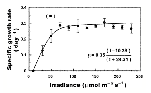
Figure 2: Representation of the hyperbola equation relating specific growth rate and irradiance levels. Temperature and salinity are kept constant (Kim et al., 2004).
Researchers emphasized a few data points as significant in understanding the link between growth rate and irradiance. Researchers found that C. polykrikoides had no growth at 10 μmolm-2s-1 and little growth at rates of 0.12 day-1 at 30 μmolm-2s-1. A threshold was also established at 90 μmolm-2s-1 where, beyond this point, any rise in irradiance did not lead to an increase in growth rate (Kim et al., 2004).
Impact of temperature and salinity
Dinoflagellate multiplies in favourable temperature and salinity conditions. By utilizing a two-factor ANOVA (Analysis of Variance), researchers found significant correlation between growth rate and temperature and salinity (Kim et al., 2004). Hence, they were able to develop the following cubic polynomial equation describing this link:
μ= b_{00}+b_{10} Τ+ b_{01} S+ b_{11} TS+⋯+b_{30} T^3+ b_{03} S^3 where μ is the specific growth rate, T is the temperature, S is the salinity, and bnn is the regression coefficients illustrating the relation between these three variables (Kim et al., 2004). This cubic equation detects potential linear and non-linear relations between the three. Using a stepwise forward regression method, researchers were able to find the following equation to describe the weight of each of the variables in accordance with a change in the growth rate:
μ= 0.946-0.177Τ-0.0474S+ 0.01218T^2+0.0026745S^2- 0.00023757T^3-0.00004003S^3
A response surface contour plot illustrates the changes in the growth rate as level curves at various values (Figure 3) (Kim et al., 2004).
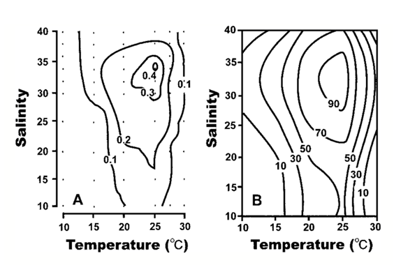
Figure 3: Response surface contour plots relating temperature and salinity to growth rate. (A) the data on the contour lines represents the specific growth rate associated with the levels of temperature and salinity. (B) the data on the contour lines represent percentages of growth rate (Kim et al., 2004).
Researchers highlighted yet again a few data points to help understand the type of relation between the variables. The organism did not grow when temperatures were under 10 ℃ and at concentrations of salt of more than 30 at 15 ℃ (Kim et al., 2004). The growth rate was at its maximum values between 21.3 and 26.2 ℃ and 27.6 and 36.7 salinity with the maximum growth rate – 0.41 day-1 — being detected at 25 ℃ and salinity 34 (Kim et al., 2004).
Understanding the impact of irradiance, temperature, and salinity on growth
Three properties describe the creation of red tides: initiation, support, maintenance, and transport. The first property states a need for a rise in population size (Kim et al., 2004, p.84). The second property states a need for suitable environmental conditions such as the ones described are needed (Kim et al., 2004). Finally, the third property states hydrologic and meteorologic forces are key in sustaining and transporting blooms.
Dinoflagellate blooms only happen under specific conditions of irradiance, temperature, and salinity. Firstly, dinoflagellates only grow at irradiance levels higher than 10 μmolm-2s-1. This can be attributed to their ability to perform photosynthesis (Kim et al., 2004). Hence, these creatures have evolved to begin growing where high quantities of irradiance can be felt. Secondly, Cochlodinium polykrikoides are theorized to be stenohaline species, i.e., species that can tolerate a narrow range of changes in salt levels (Kim et al., 2004). Salinity is crucial for processes such as osmoregulation. This microorganism has adapted to begin growing during favourable salinity conditions found in its habitat during summer. Finally, temperature is crucial for certain cellular processes as well as photosynthesis. Hence, dinoflagellate populations grow in size only at certain temperatures. In this way, dinoflagellates have evolved to grow at exponential rates when conditions favour the rapid growth of the species, leading to the creation of the red tide phenomenon.
Modelling the population dynamics of dinoflagellates and parasites from the genus Amoebophrya that infect them
Whereas some dinoflagellate species are known to be parasitic, many marine photosynthetic dinoflagellate species can themselves be infected by microparasites (Salomon & Stolte, 2010). Microparasites belonging to the genus Amoebophrya commonly target dinoflagellates as hosts(Salomon & Stolte, 2010). Amoebophrya targets a variety of dinoflagellate species; one subdivision of the Amoebophrya genus can infect over 40 different species of free-living dinoflagellates from 23 different genera (Salomon & Stolte, 2010). Infection is carried out by small flagellated dinospores. Dinoflagellates usually do not survive the infection of Amoebophrya (Salomon & Stolte, 2010). Therefore, Amoebophrya has been identified as a source of population control of dinoflagellates, and it has been suggested that they influence the geographical distribution of their dinoflagellate hosts (Salomon & Stolte, 2010). Furthermore, they can contribute to stopping harmful dinoflagellate blooms, thereby reducing the quantity of toxins produced by dinoflagellates that damage the ecosystem (Salomon & Stolte, 2010). This section will discuss the population dynamics of dinoflagellates and Amoebophrya.
Predator-prey equations
Differential equations are often used in biology to model the population dynamics of organisms. One topic frequently studied is predator-prey populations and how they affect each other. A well-known model describing predator-prey population numbers is the Lotka–Volterra model. This model is given by the following predator-prey equations (Lotka-Volterra model):
dx/dt=ax-bxy
dy/dt=dxy-cy
Where:
- x and y are the populations of prey and predator species respectively
- dx/dt and dy/dt are the instantaneous growth rates of the populations
- a,b,c,d are positive real parameters describing the interaction of the two species that are based on empirical observations and depend on the species studied.
Developing the model
Sections 4.2 and 4.3 will describe a study by (Salomon & Stolte, 2010) that looked at the population dynamics of Amoebophrya and their dinoflagellate hosts using a predation model. They based their model on the Lotka–Volterra predation model. Even though Amoebophrya are parasites of DF and not predators, the predation model was used because the infection of dinoflagellates by Amoebophrya usually ends in the termination of the dinoflagellates. However, the study made the Rosenzweig–MacArthur modification to the Lotka–Volterra predation model to account for the parasitic nature of the DF. The following ordinary differential equations were obtained for Model 1:
dH/dt=rH(1-H/K)-aH/(1+ahH) P
dP/dt=εaH/(1+ahH) P-mP
Where:
- H: the dinoflagellate host concentration (cells L-1)
- P: concentration of free-living parasitoid Amoebophrya (cells L-1)
- r: maximal reproduction rate at H=0 when the population of the DF is 0 (d-1)
- K: carrying capacity (cells L-1)
- a: search rate of Amoebophrya (dinospore-1d-1)
- h: handling time of Amoebophrya for the DF (d)
- ε: number of newly produced Amoebophrya dinospores per infected host (dinospores (killed hosts)-1)
- m: natural mortality rate of the free-living Amoebophrya dinospores (d-1)
The rate of change dH/dt is given by the reproduction rate of the host dinoflagellates minus the infection rate of dinoflagellates by Amoebophrya. The reproduction rate of host dinoflagellates is a logistic function. The infection rate depends on both the concentration of dinoflagellate host and the concentration of parasitoids. In other words, the more dinoflagellates and Amoebophrya there are, the higher the infection rate is. Notice how the infection rate decreases when the handling time h increases because the parasite spends more time inside its host, where it is not infecting other hosts.
The rate of change dP/dt is given by the infection rate minus the natural death rate of Amoebophrya. However, the infection rate also depends on . This makes sense since the more Amoebophrya dinospores are produced for each host infection, the more parasitoids will be present in the water that can infect host dinoflagellates.
Most Amoebophrya data in natural samples is in the form of the percentage of infected dinoflagellate hosts. To improve the comparison between the model outcomes and the field data, a modification to the differential equation must be made to model more explicitly and accurately the infected host stage (red potion of the equation). The more accurately the infection stage is modelled, the better the predictions that can be made. A state variable , representing the number of infected hosts, was introduced. The following modified differential equation for the rate of change of the Amoebophrya concentration was obtained:
dP/dt=ε I/H-mP
Where the derivative of the number of infected hosts I is given by:
dI/dt=aH/(1+ahH) P-I/H
Along with the original differential equation for the rate of change of the concentration of dinoflagellates hosts (shown below), the set of modified equations make up Model 2.
dH/dt=rH(1-H/K)-aH/(1+ahH) P
Values for the different parameters of model 1 and model 2 were found in experimental data or estimated from studies. Simulations of the models were run with three different dinoflagellate species and the respective Amoebophrya species that can infect them. The simulations were compared to experimental data to test the validity of the models. The following graphs from Figure 4 give an example of the accuracy of the model in predicting population dynamics.
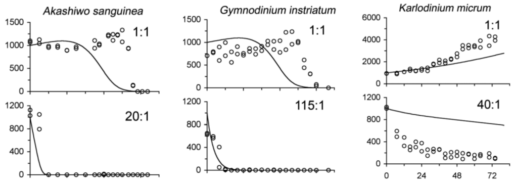
Figure 4: Simulation using Model 2 of concentration of uninfected dinoflagellate hosts (cells ml-1) as a function of time (h) for dinoflagellate species Akashiwo sanguinea, Gymnodinium instriatum, and Karlodinium micrum. The ratios (e.g. 1:1) indicate the ratio of dinospores to host dinoflagellates. The carrying capacity K was set to 1 × 10⁷ cells L-1 for Akashiwo sanguinea, 5 × 10⁶ cells L-1 for Gymnodinium instriatum, and 2 × 10⁷ cells L-1 for Karlodinium micrum. Open circles represent experimental data and solid lines are the model 2 simulations.
From Figure 4, the concentration of uninfected dinoflagellate cells generally decreases quicker as the ratio of dinospores to dinoflagellates increases: there are more dinospores that can infect a dinoflagellate per dinoflagellate. Initial conditions were set according to experimental data from previous studies. Overall, the models agreed generally well with the experimental data, showing that the model could be used to predict population dynamics of Amoebophrya and dinoflagellates. Of course, the model is not perfect. In nature, there are countless variables affecting population dynamics that are not considered in the models. However, the model does offer a general approximation of the population dynamics of these two organisms and provides a useful tool for predicting how populations will change with time and differing conditions.
Carrying capacity
For dinoflagellates to coexist with Amoebophrya in a stable manner, their carrying capacity must be within certain limits. Carrying capacity may be indicative of the trophic state of the water body. The lower bound of carrying capacity is the critical carrying capacity Kc, which represents the minimum carrying capacity of dinoflagellates required for dinoflagellates to coexist in a stable manner with Amoebophrya. KC given by:
K_C=m/(a(ε-mh))
The upper bound of carrying capacity is KS, which is given by:
K_S=(ε+mh)/(ah(ε-mh))
If the carrying capacity K is smaller than the critical carrying capacity KC, then there is no stable state of coexistence with Amoebophrya. If K is larger than KS, coexistence is possible but is unstable; dinoflagellate and Amoebophrya populations will fluctuate like Lotka–Volterra oscillations (Figure 5).
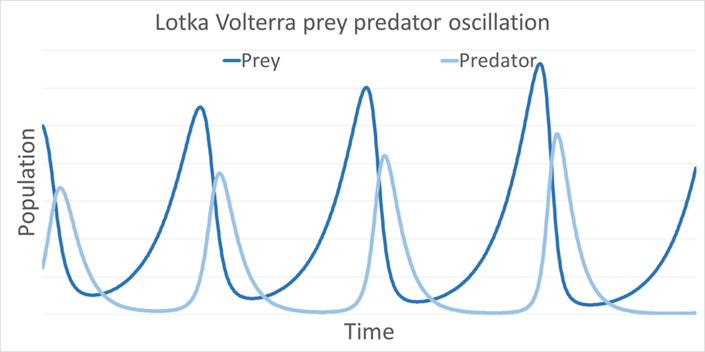
Fig. 5. Example of Lotka–Volterra oscillations (Lange et al., 2016).
When KC < K < KS, then stable coexistence between dinoflagellates and Amoebophrya can occur (Figure 6). The following graphs are Model 2 simulations representing how their population fluctuates according to the carrying capacity.
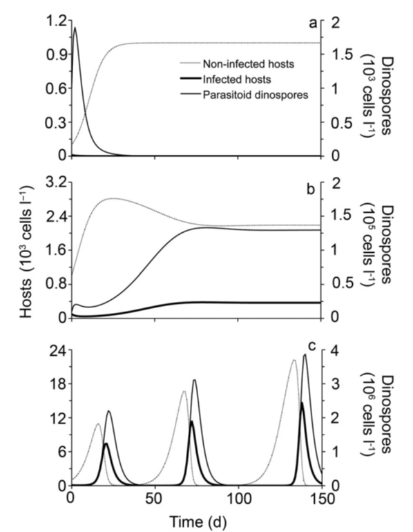
Figure 6: 150-Day Simulation using Model 2 of Population Dynamics Between Akashiwo sanguinea and Its Amoebophrya parasitoid at varying K values. In (a), K < KC; in (b), KC < K < KS; in (c), K > KS.
We see from graph (a) that when K < KC, there is no stable state of coexistence between dinoflagellates and Amoebophrya. Parasitoid numbers are near zero, so there are little to no infected dinoflagellates. In graph (b), when KC < K < KS, dinoflagellates and Amoebophrya undergo stable coexistence. Cell concentrations of infected hots, non-infected hosts, and parasitoid dinospores undergo fluctuations at the start of the simulation but eventually reach a stable equilibrium. Finally, in graph (c), when K > KS, dinoflagellate populations fluctuate according to Lotka–Volterra oscillations. The species coexist but unstably.
Conclusion
Dinoflagellates’ vertical motion can be modelled with equations relating to their nitrogen-to-carbon uptake rates, their growth and respiration, and photosynthesis. Dinoflagellates have a specific carbon-to-nitrogen ratio to ensure their best chances of survival, and they adjust when to surface for photosynthesis based on how much nitrogen it has. If it does not have nitrogen, then it does not surface, as it cannot perform photosynthesis efficiently. When it has an abundance of nitrogen, it surfaces and performs photosynthesis efficiently. This solution allows the dinoflagellate to optimise its energy expenditure, and only perform energy-intensive tasks like surfacing when necessary.
Dinoflagellates are responsible for red tide phenomena. These creatures begin as cysts dormant on the ocean floor and germinate when conditions are favourable. Throughout their evolutionary trajectory, dinoflagellates have undergone intricate adaptations, including the development of sophisticated internal clock mechanisms, driven by the necessity to survive and thrive in ever-changing aquatic environments. The evolution of these internal clocks can be attributed to the selective pressures imposed by cyclic and unpredictable environmental factors, notably light availability, temperature fluctuations, and nutrient variations. Over time, dinoflagellates evolved regulatory systems to synchronize their biological processes with diurnal and seasonal changes, optimizing critical life cycle events such as encystment, dormancy, and germination. The emergence of these internal clocks likely conferred adaptive advantages, enabling dinoflagellates to anticipate and respond to environmental cues, thereby enhancing their survival strategies.
Until resources are depleted, germinated dinoflagellates reproduce at exponential rates by asexual fission, leading to the red tide phenomena. This organism has evolved to begin this rapid growth during conditions that favour its cellular processes such as photosynthesis and osmoregulation. However, these favourable conditions are not present all year round. At low rates of irradiance and temperature and high rates of salinity, these creatures cannot reproduce or survive as swimming dinoflagellates. Hence, nature has enabled this microorganism the ability to survive these periods as cysts sitting at the bottom of the ocean, waiting for the next wave of favourable environmental conditions.
Finally, population dynamics between dinoflagellates and the parasites from the genus Amoebophrya that are known to infect them can be modeled using differential equations. Amoebophrya has been identified as a source of population control of blooming toxic dinoflagellates. Overall, the simulations ran with the model generally agreed with experimental data, making it a useful tool in predicting the population dynamics of these two organisms.
References
Anderson, D. M. (1998). Biology of the red tide dinoflagellate, Alexandrium fundyense: Ecophysiological aspects of cyst formation and germination. In Physiological Ecology of Harmful Algal Blooms (pp. 147-168). Springer.
Anderson, D. M., Keafer, B. A. (1987). An endogenous annual clock in the toxic marine dinoflagellate Gonyaulax tamarensis. Nature, 325, 616–617.
Anderson, D. M., Lindquist, N. L. (1985). Time-course measurements of phosphorus depletion and cyst formation in the dinoflagellate Gonyaulax tamarensis Lebour. Journal of Experimental Marine Biology and Ecology, 86, 1–13.
Anderson, D. M., Aubrey, D. G., Tyler, M. A., Coats, D. W. (1982). Vertical and horizontal distributions of dinoflagellate cyst in sediments. Limnology and Oceanography, 27, 757–765.
Anderson, D. M., Kulis, D. M., Doucette, G. J., Gallager, J. C., Balech, E. (1994). Biogeography of toxic dinoflagellates in the genus Alexandrium from the northeast United States and Canada as determined by morphology, bioluminescence, toxin composition, and mating compatibility. Marine Biology, 120, 467–478.
Anderson, D. M., Fukuyo, Y., Matsuoka, K. (2003). Cyst methodologies. In G. M. Hallegraeff, D. M. Anderson, A. D. Cembella (Eds.), Manual on Harmful Marine Microalgae (Monographs on Oceanographic Methodology 11, pp. 165–190). UNESCO.
Anderson, D. M., Taylor, C. D., Armbrust, E. V. (1987). The effects of darkness and anaerobiosis on dinoflagellate cyst germination. Limnology and Oceanography, 32, 340–351.
Bewley, J. D., & Black, M. (1982). Physiology and biochemistry of seeds in relation to germination: Volume 2: Viability, dormancy, and environmental control. Springer Science & Business Media.
Cullen, J. J., & Horrigan, S. G. (1981). Effects of nitrate on the diurnal vertical migration, carbon to nitrogen ratio, and the photosynthetic capacity of the dinoflagellate Gymnodinium splendens. Marine Biology, 62(2), 81-89. https://doi.org/10.1007/BF00388169
Heaney, S. I., & Eppley, R. W. (1981). Light, temperature and nitrogen as interacting factors affecting diel vertical migrations of dinoflagellates in culture. Journal of Plankton Research, 3(2), 331-344. https://doi.org/10.1093/plankt/3.2.331
Ji, R., & Franks, P. J. S. (2007). Vertical migration of dinoflagellates: model analysis of strategies, growth, and vertical distribution patterns. Marine Ecology Progress Series, 344, 49-61. https://www.int-res.com/abstracts/meps/v344/p49-61/
Keafer, B. A., Buesseler, K. O., Anderson, D. M. (1992). Burial of living dinoflagellate cysts in estuarine and nearshore sediments. Marine Micropaleontology, 20, 147–161.
Kim, D.-I., Matsuyama, Y., Nagasoe, S., Yamaguchi, M., Yoon, Y.-H., Oshima, Y., Imada, N., & Honjo, T. (2004). Effects of temperature, salinity and irradiance on the growth of the harmful red tide dinoflagellate Cochlodinium polykrikoides Margalef (Dinophyceae). Journal of Plankton Research, 26(1), 61-66. https://doi.org/10.1093/plankt/fbh001
Lange, P., Weller, R., & Zachmann, G. (2016). Knowledge Discovery for Pareto Based Multiobjective Optimization in Simulation. https://doi.org/10.1145/2901378.2901380
Lotka-Volterra model. The University of Queensland Retrieved November 28 from https://teaching.smp.uq.edu.au/scims/Appl_analysis/Lotka_Volterra.html#:~:text=The%20Lotka%2DVolterra%20equations%20x,as%20a%20predator%20and%20the
Martin, J. L., Wildish, D. J. (1994). Temporal and spatial dynamics of Alexandrium cysts during 1981–84 and 1992 in the Bay of Fundy. In R. Forbes (Ed.), Proceedings of the Fourth Canadian Workshop on Harmful Marine Algae (pp. 2016). Canadian Journal of Fisheries and Aquatic Sciences.
Matrai, P. A., Keller, M. D., & Anderson, D. M. (2005). The single-cell stage and mitotic cell cycle of the dinoflagellate Alexandrium fundyense (Dinophyceae). Phycologia, 44(1), 41-55.
Matrai, P., Thompson, B., Keller, M. (2005). Alexandrium spp. from eastern Gulf of Maine populations: Circannual excystment. Deep-Sea Research II. [doi:10.1016/ j.dsr2.2005.06.013]
Rengefors, K., Anderson, D. M. (1998). Environmental and endogenous regulation of cyst germination in two freshwater dinoflagellates. Journal of Phycology, 34(4), 568–577.
Salomon, P. S., & Stolte, W. (2010). Predicting the population dynamics in <em>Amoebophrya</em> parasitoids and their dinoflagellate hosts using a mathematical model. Marine Ecology Progress Series, 419, 1-10. http://www.jstor.org/stable/24874340
Scholin, C. A., Hallegraeff, G. M., Anderson, D. M. (1995). Molecular evolution of the Alexandrium tamarense ‘‘species complex” (Dinophyceae): dispersal in the North American and West Pacific regions. Phycologia, 34, 472–485.
Stock, C. A., McGillicuddy Jr, D. J., & Anderson, D. M. (2005). Evaluating hypotheses for the initiation and development of Alexandrium fundyense blooms in the western Gulf of Maine using a coupled physical–biological model. Deep Sea Research Part II: Topical Studies in Oceanography, 52(19-21), 2522-2542.
U.S. National Office for Harmful Algal Blooms. (n.d.). Dinoflagellate Life Cycle. Retrieved 10/2/2023 from https://hab.whoi.edu/about/
Wheatcroft, R. A., Martin, W. R. (1996). Spatial variation in short-term (super(234)Th) sediment bioturbation intensity along an organic-carbon gradient. Journal of Marine Research, 54(4), 763–792.
White, A. W., Lewis, C. M. (1982). Resting cysts of the toxic, red tide dinoflagellate Gonyaulax excavata in Bay of Fundy sediments. Canadian Journal of Fisheries and Aquatic Sciences, 39, 1185–1194.
Yamaguchi, M., Itakura, S., Imai, I., Ishida, Y. (1995). A rapid and precise technique for enumeration of resting cysts of Alexandrium spp. (Dinophyceae) in natural sediments. Phycologia, 34, 207–214. Zheng, Q., & Klemas, V. V. (2018). 8.04 – Coastal Ocean Environment. In S. Liang (Ed.), Comprehensive Remote Sensing (pp. 89-120). Elsevier. https://doi.org/https://doi.org/10.1016/B978-0-12-409548-9.10518-4