Exploring Aquatic Fungi Through Mathematical Tools

Izabela Junqueira Magalhaes, Kristina Kerkelova, Ruizhi Liu, Yasmine Sadr Kaufmann

Abstract

The beauty of mathematics lies in its ability to create models to simplify complex things in real life and give explanations to them. Models are a great way to study and analyze species in nature and it is the same for aquatic fungi. Mathematical models also help us predict their behavior based on various factors. The logistical model to predict populational growth for aquatic fungi will be introduced first, followed by models for their spatial distribution based on their diversity. Some aquatic fungi can have fatal effects on amphibians, and a model to describe the spread of a particular disease, chytridiomycosis, is introduced next. This model displays the effect of the inoculation of a particular bacterium in the spread of chytridiomycosis. Aquatic fungi have been known for their ability to decompose plant litter in nature, and this process will be described by mathematical models. Models will also be applied to explain bioremediation processes. Then, models linking the relationship between the shape of the hyphal tip and fungal growth will be shown, together with the models for the growth of mycelium in fungi.

Introduction

Mathematics and biology are two fields that are strongly related. From populational modeling and the analysis of different structures and their properties to new approaches such as disease modeling and data analysis of DNA sequences, this intersection can offer valuable information about the complexity of biological systems (Allman & Rhodes, 2004). In this context, there is no doubt about the importance of biomathematics and its wide range of applications. When studying aquatic fungi and their many features and characteristics, this field can help scientists better understand this still mysterious but widely fascinating species.

In this essay, we will discuss different features of aquatic fungi that can be studied through mathematical approaches such as modeling to analyze their populational dynamics, diversity, and spatial distribution, as well as their growth. Moreover, chemical processes such as leaf decomposition and the interactions of aquatic fungi species with other organisms will be studied using mathematical tools. The branching pattern of their hyphae will also be put under analysis to discuss their complexity and amazing organization.

Among the applications of this interdisciplinary study, the understanding that biomathematics can offer about specific populations, species, and ecosystems has a wide range, such as unraveling intricate biological systems, predicting outcomes, and testing hypotheses. Thus, these tools can be used to better understand their dynamics, assess the health of the ecosystems for conservation and management purposes, and get ecological insights into the complex relations and adaptations within species or between them, as well as make predictions of growth and environmental impacts on populations given certain conditions.

Mathematical models

Mathematical models have great importance in biology since they provide a way to represent, simulate, and analyze various processes within populations and ecosystems. Mathematically modeling the behavior of organisms is a hard task, since multiple factors must be accounted for and the interactions between organisms and the variables that play roles in ecosystems are complex. Thus, the first step to constructing a model to describe a biological phenomenon is following the scientific method and having a clear question to drive the approach (Dym, 2004). It is important to know that models are not perfect representations of reality, but tools that can be used to better understand it. The first formulation of a model constructed is then analyzed and continuously adapted to better represent the situation being analyzed, as seen in the Figure. 1:

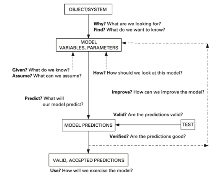
Figure 1: Schematic overview of the formulation and development of a mathematical model (Dym, 2004).

Populational growth modeling of aquatic fungi

Populational growth modeling is a key mathematical approach to represent and analyze changes in the sizes and behaviors of different species populations over time. In the context of aquatic fungi, this is extremely important to better understand their ecology and the different factors that affect their growth and equilibrium. As we know, fungi are extremely versatile and adaptable to many different environments. Thus, studying their populational growth under different conditions and environments can help scientists not only understand their evolution and adaptations but also help the construction of models inspired by their adaptability with other applications.

Due to the formation of fungal colonies and their ability to function in a decentralized fashion, responding to local changes in context while also interacting on a broader scale within the colony and with other organisms, models based on the study of their populational growth and interactions are great inspirations for management strategies of large communication algorithms, complex artificial networks, and distributed urban planning and infrastructure improvement plans, for example (Falconer et al., 2010).

So far, most studies done with the goal of modeling fungal colonies have focused on terrestrial species, especially those decomposing plant litter in florets or growing on food. The analysis of those models, however, can help in the preliminary formulation of models to analyze the behavior of aquatic species of fungi as well. In most models, factors such as temperature, pH, humidity, nutrient availability, and various dynamics with other species are considered to model populational growth and the occupation of habitats by fungi (Dantigny, 2021; Shi & Wang, 2022).

By having these parameters in mind and adapting them to the context of aquatic environments, and thus analyzing the water temperature, salinity, pH, the currents of water, nutrient availability such as in plant litter and wood, and also the presence of other species such as algae and bacteria in co-occurrence relations (Krauss et al., 2011; Vass et al., 2022), we can begin to formulate models to better understand the aquatic fungi growth and development. One model that is commonly used by scientists to study populational dynamics of different species is the logistic model.

The logistical model is used to predict populational growth over time based on the environmental capacity and resources. It is an extension of the exponential growth model but introduces a carrying capacity, representing the maximum population size that an environment can sustain. The model is expressed through a differential equation, where the rate of population growth is proportional to both the current population size and the difference between the carrying capacity and the current population. This model is particularly relevant in understanding population dynamics when resources are limited and analyzing their adaptations to environmental constraints.

Applying the logistical model to model aquatic fungal populations involves considering the aforementioned factors such as nutrient availability, space, and other ecological conditions affecting fungal growth to determine the environmental capacity (usually expressed as K). Furthermore, we have the variable N, which represents the size of the population, and t, which represents time. The growth is given by the variation of the population over time, thus dN/dt. Lastly, in this model, we also have r, the populational growth capacity, which reflects how fast the population will achieve its equilibrium value and what will be the reaction time to go back to it if disturbed, and the parameter “a“, which varies based on the population size “N” and signifies the curve's relative position to the origin. We can visualize the model in the following equations (Shi & Wang, 2022):

Populational change: $\frac{dN}{dt} = rN\left(1 - \frac{N}{K}\right)$

Equation 1: Populational change.

Integral formula: $N_t = \frac{K}{1 + e^{a - n}}$

Equation 2: Integral formula.

In the equation, we can analyze that during the initial phase might exhibit rapid fungal population expansion, like exponential growth. However, as resources become constrained, the population growth slows down, eventually reaching a stable equilibrium known as the carrying capacity. This capacity reflects the maximum number of aquatic fungi the ecosystem can support sustainably. Mathematically, this is modeled by having a small “n” in the initial phase, plus the ratio “N / K” is also small, causing (1-N / K) to approximate 1. During this stage, the inhibitory effect is negligible, and the population grows geometrically, represented as rN. As “n” increases, the inhibitory effect becomes more pronounced until, at “n = k,” (1-N / k) becomes (1-k / R), equaling 0 (Shi & Wang, 2022). At this point, population growth ceases, and the population stabilizes at a constant size, establishing an equilibrium, as we can see in Figure 2.

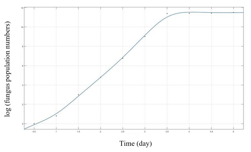
Figure 2: Example of the growth curve of an aquatic fungal species based on the logistic model (Shi & Wang, 2022).

By using the logistical model, researchers and ecologists can gain insights into how aquatic fungal populations respond to environmental changes and resource fluctuations, aiding in the development of strategies for sustainable aquatic ecosystem management. However, this model is not very specific to aquatic fungal species, and it can be improved and specified to take more factors into account and better reflect the ecological dynamics in which they are involved.

An example of restriction to the model is the competition between species. To overcome this limitation, scientists also have a model called the Lotka-Volterra model, which is an extension of the general logistic model that accounts for interspecific competition by introducing a competition coefficient β:

Ppopulational change for each species: $\frac{dN_i}{dt} = r_i N_i \left(1 - \frac{N_{i}}{K_{i}}} - \beta \frac{N_{k}} {K_{k}}\right)$

Equation 3: Populational change per species.

Ni is the species under analysis and N_K is the competitor. In this model, one of the species can eliminate the other one, or they can both coexist, reaching an equilibrium state. Appropriate modelling of both populations' behaviour requires the study and analysis of the two species.

This is only one example of different adaptations and improvements to models that can used to study the populations of aquatic fungi. With more research done about these wonderful organisms and their many ecological interactions, better models can be constructed to gain essential information about these incredibly important and complex species.

A mathematical model of the spread of chytridiomycosis

Chytridiomycosis is a disease caused by a parasitic aquatic fungi that primarily affects amphibians. Chytridiomycosis is caused by the fungus Batrachochytrium Dendrobatidis (Bd). Bd has unfortunately been the cause of death of many frogs over the years, reducing and preventing regular skin function, leading to deaths due to cardiac arrest (Ackleh et al., 2016). Some scientists have even gone so far as to call the infection and spread of Bd among amphibians an epidemic, as large populations of frogs are killed by chytridiomycosis and it is a pathogen that spreads very easily among frog populations, even leading to some local extinctions of frog populations (Briggs et al., 2010).

Interestingly, however, different frog populations, despite being of the same species, have reacted differently to chytridiomycosis. While some populations have gone extinct, others have consistently been able to survive infection, with a much lower concentration of adult frogs contracting the disease (Briggs et al., 2010). In certain models, however, population extinction was found to occur 61% of the time in the long-term, after infection by Bd, indicating that, if nothing is done to prevent it, chytridiomycosis would often lead to the death of frog populations (Harer, 2014).

Different approaches have been taken to study the effect of Bd on frog populations, with different mathematical models and simulations. The models aim to find a way to aid frogs in surviving the disease and accurately depict how the disease spreads and the effect chytridiomycosis will potentially have on a frog population. Specifically, many models examine the environmentally specific characteristics that led to an increased survival rate of infected frogs. One such characteristic that is believed to increase the survival rate of frogs is the frog being inoculated with the bacteria Janthinobacterium lividum (Jl) (Ackleh et al., 2016).The inhibition of the spread of Bd by Jl is an interesting weakness that Batrachochytrium Dendrobatidis has. Like all chytrids, Bd has many design solutions to ensure spore dispersal and adherence to substrates, but it is not able to persevere against the fungicide Jl produces. Some frogs have incorporated this design solution against Bd, where Jl, the enemy of Bd, is their friend. This weakness to fungicides, while limiting the spread of Bd, is also an interesting indication of the balanced state of the natural world, with nothing being invulnerable.

A model on the effect of inoculation with Janthinobacterium lividum

A study published in 2016 produced a mathematical model of a frog population infected with Bd and used it to determine the effect of inoculation with Janthinobacteriumlividum and varying temperaturein decreasing the transmission of chytridiomycosis. Jl mitigates the spread of Bd by producing violacein, a fungicide that inhibits Bd growth. Evidence of the effect of Jl inoculation was seen when a frog species, Rana muscosa, was exposed to Jl and then infected with Bd. The frogs showed a much higher survival rate and lower rate of Bd infection. The mathematical model created attempts to determine when and how often, precisely, frogs should be inoculated with Jl, to best ensure their survival. The model also studies the importance of temperature in disease transmission and proliferation. The importance of temperature was considered as it was found that Bd grew less on frogs consistently in an environment above 28 °C and that above 32 °C the entire fungal population died within 96 hours (Ackleh et al., 2016).

Certain assumptions were made in order to create a model of a frog population. It was assumed that the frog population was in a single pond, that the population was divided into frogs and tadpoles, that frogs only infected frogs and tadpoles only infected tadpoles, that tadpoles with Jl are protected against Bd, that inoculation with Jl only lasts for a limited amount of time and that all frogs infected with Bd die. A diagram was made of the mathematical model created as seen in Figure 3. It is important to go over all these assumptions, as they indicate potential sources of error in the mathematical model created and why the model may not necessarily reflect reality, due to the many generalizations (Ackleh et al., 2016).

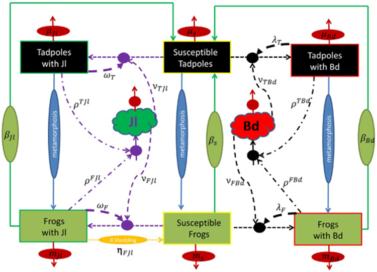
Figure 3: Flow diagram of the mathematical model of chytridiomycosis. Transmission is simulated between two stages (tadpoles and frogs) with Bd fungus and Jl bacteria. Solid lines represent vital rates; dashed lines represent transmission rates; dashed-dotted lines represent zoospore release rates; dotted line represents the shedding rate (Ackleh et al., 2016).

Multiple hyperbolic differential equations were used to map out the relations between these different subsets of the frog population, those susceptible to the disease, those inoculated with Jl, and those with Bd. Some of the equations used were R(t) = R_s(t) + R_Jl(t) + R_Bd(t), where R(t) is the total population of frogs, and the subscript indicates the populations of frogs of each subset. The total population R(t) is determined by integrating the density of each population, with a separate equation being used to determine the densities. The densities of the populations were expressed with F(x, t) with subscripts again indicating if the frog or tadpole was susceptible (s), infected (Bd), or inoculated (Jl) (Ackleh et al., 2016).

The following system of partial differential equations (Equation 4) was used in the calculations of the frog population. The term λ_F(x, t)F_s(x, t) is used to indicate the infection rate because of skin contact and ν_FBd(x)Bd(t)F_s indicates the infection rate due to the presence of chytrid zoospores in the environment. Since only the susceptible populations can contract Bd in this model, only the density of the susceptible populations is multiplied in. The symbol g denotes the growth rate and ω_Fdenotes the ability of a group of frogs to be inoculated with Jl, depending on its size. All these formulas work together to represent a mathematical simulation of the spread of chytridiomycosis (Ackleh et al., 2016).

$\begin{align* } \frac{\partial}{\partial t} F_s + \frac{\partial}{\partial x} (g_s F_s) + m_s F_s &= -\lambda_F (x,t) F_s(x,t) - \omega_F (x,t) F_s(x,t) - v_F B_d(x) B_d(t) F_s(x,t) - v_F J_l(x) J_l(t) F_s(x,t) + \eta_F J_l(x,t) F_{Jl} \\ \frac{\partial}{\partial t} F_{Bd} + \frac{\partial}{\partial x} (g_{Bd} F_{Bd}) + m_{Bd} F_{Bd} &= \omega_F (x,t) F_s(x,t) + v_F J_l(x) J_l(t) F_s(x,t) - \eta_F J_l(x,t) F_{Jl} \end{align* }$

Equation 4: A portion of the calculations to create the model of a frog population with both Jl and Bd present and competing (Ackleh et al., 2016).

With the model created, three different types of scenarios were tested, a control scenario, with neither Bd or Jl, a scenario with only Bd, and a scenario with both Bd and Jl present. For each type of scenario, simulations were made at different temperatures corresponding to different locations and climates in the United States. The models indicated that the best time to inoculate with Jl is during the frogs' breeding season and that chytridiomycosis does not proliferate well in locations with higher average temperatures, thus making the frogs in warmer climates more likely to survive if infected. Unfortunately, the amount of Jl required to inoculate a large population of frogs could cause other damage to the ecosystem, so it is not a perfect solution to the chytridiomycosis epidemic among frogs, but it is a possible solution (Ackleh et al., 2016).

Models for decomposition by aquatic fungi

As described in the previous paper, aquatic fungi are excellent plant litter decomposers and play a crucial role in the aquatic food web. Through their composition abilities, they gain energy, grow their biomass, and pass energy to other trophic levels in the food web (specifically to macroinvertebrates that do not possess the enzymes needed to digest plant matter). Simple mathematical models can be used to describe decomposition by aquatic fungi, and how it increases fungal biomass.

Colonization of plant matter by aquatic fungi is the first step in decomposition. Barlocher (1980) aimed to model the number of fungi colonizing plant litter (the substrate). In his study, he placed fine and coarse-meshed bags filled with plant matter (oak leaves, larch, or spruce needles) into various steams and recorded the fungal count (see Figure 4). The fine-meshed bags would allow access to only the fungi and other decomposers, while the coarse–meshed bags would allow both fungi and macroinvertebrates to access the substrate (Bärlocher, 1980).

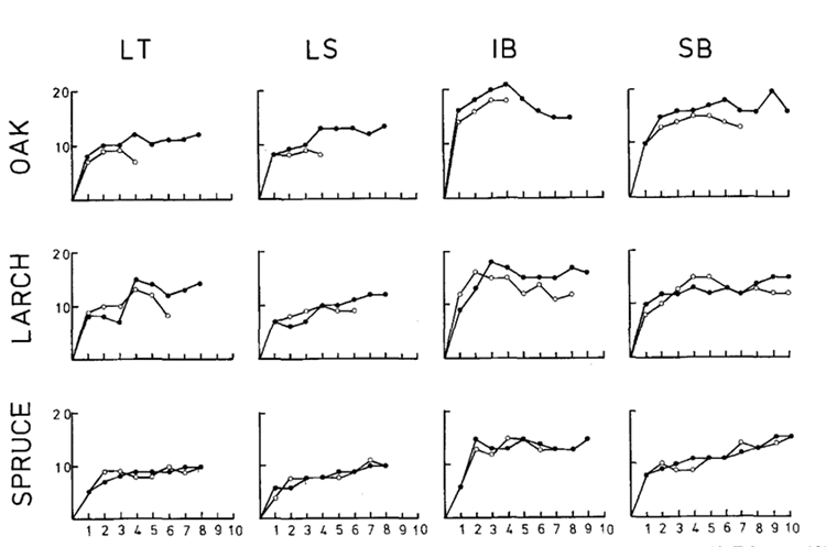
Figure 4: Fungal species count on various substrates (oak leaves, larch, and spruce needles) over 10 weeks (about 2 and a half months). The darker line represents the fungal species count in fine-meshed bags (fungal access only), and the lighter line represents the fungal species count in coarse-meshed bags (fungal and macroinvertebrate access). LT, LS, IB, and SB represent the names of the four streams where the study was conducted (Bärlocher, 1980).

Barlocher (1980) observed that substrates in fine-meshed bags had more abundant fungal colonization as opposed to substrates in coarse-meshed bags, likely due to the predation of fungi by macroinvertebrates. He also observed that oak and larch substrates decay much faster than spruce when in coarse-meshed bags, as seen in Figure 4 above where the oak substrate is almost always gone before the halfway point in the study (Bärlocher, 1980).

The number of species in the fine-meshed bags follows a similar pattern with all substrates in all streams: they increase until reaching a stable plateau. This indicates that at a certain point, all possible parts of the substrate have been colonized, meaning that if new fungi enter, old fungi must leave to maintain a balance. The rate of turnover decreases eventually (Bärlocher, 1980).

Feeding by invertebrates can only happen once decomposition has taken place. More feeding activity by invertebrates results in a decrease in substrate weight, leading to a decrease in fungi count. Therefore, the weight of a substrate can indicate how much decomposition has occurred, and how much fungi was present on the substrate before it was consumed by other predators (Bärlocher, 1980).

Barlocher's findings can be used to estimate the loss of substrate weight over time by fitting his observations to the decay function (Equation 5).

$W(t) = W(o) e^{-kt}$

Equation 5: Decay function for weight of substrate when exposed to aquatic fungi decomposition, where W_(t) is weight at time t, W_(o) is weight at the start of the experiment, k is a decay constant particular to the type of substrate, and t is time in days (Bärlocher, 1980).

Another way to model decomposition is by calculating the amount of substrate available for colonization, which can be expressed as the area under the decay curve using Equation 6 below.

$S = k \cdot A^{z}$

Equation 6: S = number of species at the end of the experimental period, A is the area below the decay curve, representing the area available for colonization, k is a substrate-specific constant, and z = 0.47 (Bärlocher, 1980).

With the Equation 6 above, the number representing fungal biomass on a particular substrate after a particular time (dependent on A), can be obtained. Both above models show that increased predation by macroinvertebrates decreases substrate weight, and as a result, fungal biomass (Bärlocher, 1980).

The more space available, the more fungi on the substrate. One clever design solution that aquatic fungi have developed is the ability to use every bit of the resource that they have access to, as shown in Equation 6. They optimize the amount of nutrients obtained from a single source.

Models for bioremediation

In the previous chemistry paper, aquatic fungi's ability to degrade organic pollutants was described. In short, through their enzymatic activities, aquatic fungi can break down many compounds including oils, gasoline, dyes, pesticides, and herbicides (Thacharodi et al., 2023). Aquatic fungi's ability to break down organic pollutants is an example of bioremediation.

Fungi break down dyes by cleaving the bonds that keep them together, rather than breaking down dyes partially and leaving toxic fragments behind. Enzymes involved in this breakdown are non-specific and can break down other pollutants as well.

Goyal et al.'s non-linear mathematical model (Equations 7-10, below) aims to show the rate at which aquatic fungi can help remove organic pollutants, specifically dyes, with the level of degradation depending on the concentration of pollutant and fungal population density (2014). In their study, they consider four variables: concentration of dye, fungal population density, concentration of nutrients, and concentration of dissolved oxygen (Goyal et al., 2014). Goyal et al.'s model uses fundamental concepts from the Michaelis-Menten Kinetics model, which explains how reaction rates depend on the concentration of enzyme and substrate present (Cornish-Bowden, 2015).

$\frac{dT}{dt} = -Q - \alpha_0 T - \frac{kmT}{k_{11} + k_{12}T} \qquad \qquad(7)$

$\frac{dm}{dt} = q - \frac{\pi kmT}{k_{11} + k_{12}T} - \alpha m + k_{1}mn \qquad \qquad(8)$

$\frac{dn}{dt} = q_1 - \alpha_{1}n - k_{1}mn \qquad \qquad (9)$

$\frac{dC}{dt} = q_2 - \alpha_2 C - \lambda k_{1}mn - \frac{\lambda kmT}{k_{11} + k_{12} T} \qquad \qquad (10)$

Equations 7-10: Goyal et al.'s model describing the rate of breakdown of organic pollutants (dyes) by aquatic fungi (Goyal et al., 2014).

In equations 7 to 10 above, T is the concentration of dyes present in water, with the dyes being discharged into the water at rate Q. m is the density of fungal biomass responsible for the breakdown, growing at rate q. n is the concentration of nutrients available, supplied at a constant rate q₁. C is the concentration of dissolved oxygen, supplied at a constant rate q₂. α, α₁, α₂, and α₃, are natural depletion coefficients of organic pollutants, fungal population, nutrients, and dissolved oxygen respectively. k is a rate of depletion coefficient caused by the interactions between pollutants and fungi. k₁₁ and k₁₂ are constants defining the Michaelis-Menten kinetics model. π, 𝜆_1,and 𝜆₂are proportionality constants that are between zero and one.

This model can be applied to two cases: (1) the rate at which pollutants are discharged into the water is constant and the rate of fungal growth is also constant – in this case, fungi are working efficiently to break down pollutants. (2) the rate at which pollutants are discharged is constant, but the rate at which fungi grow is zero – in this case, fungi would break down pollutants for a finite time or until they die. Since no growth is happening, eventually there would be more pollutants than fungi.

When there is enriched growth (the rate of fungal growth is higher than that of pollutant discharge), the fungi would make significant strides in breaking down all dye present. Also, when there are more pollutants to break down (up to a certain limit), the fungi will grow as they benefit from the breakdown since they gain nutrients from this process. This is an example of a design solution as the fungi are fully taking advantage of all of the nutrients available to grow their biomass.

Mathematical Analysis of Aquatic Fungi's Structures and Growth

Aquatic fungi hyphae growth is an important aspect for researchers to study since hyphae play such an important role in releasing exoenzymes for digestion and ingestion of food through osmosis. The three-dimensional network of mycelium composed of hyphae will maximize its surface for absorbing nutrients and for more efficiently colonizing the substrates (Künzler, 2018). Therefore, there have been many mathematical models created to describe the relationship between various aspects of aquatic fungi, like the shape of the hyphal tip, hyphal branching, and fungal growth. However, one thing that needs to be kept in mind is that for all the modelling approaches, it is the description between theoretical predictions and experimental data. The model itself does not explain any mechanism of hyphal growth and may not be applicable for other organisms or if the experiment is conducted under different growth conditions (Prosser, 1995).

Fungal growth and shape of hyphal tips

There have been studies generating models to explain the relationship between the shape of hyphal tips and applied mathematical models to describe fungal growth. Hypha extends at the hyphal tip and vesicles are transported to the extension zone to be incorporated in that region. The region is also responsible for the direction of hyphae growth and responds to external stimuli. The early model proposed by Green and King to describe this relation is given by equation 11 below:

$\frac{dm}{dt} = \frac{A r^k}{R}$

Equation 11: The equation proposed by Green and King to describe the tip growth for the alga Nitella (Prosser, 1995).

The m is the distance from the apex, so the left part represents the rate of hyphae expansion. The A on the right is a constant. In this model, the tip of the hypha is assumed to be hemispherical, and it is the same as the radius, R, of the cylindrical hypha. The r is the radius at a chosen point from the cell wall of the extension zone. The r is 0 if it is at the apex of the hyphae and is R for the maximum radius, the same as the radius for the hemispherical tip. The expansion is thought to be the change in a small circular region at the cell wall, as the materials released by the vesicles move outwards from the hyphal central longitudinal axis. The hypha is said to be isotropic if growth in both longitudinal and meridional planes occurs equally, and anisotropic otherwise. The isotropic growth would result in circular shapes, which remain the same as the expansion shape. The degree of difference in the two planes, i.e. anisotropy, is quantified by the allometric coefficient K, which is the ratio of the growth rate in the meridional axis over the growth rate in the longitudinal axis. K can be adjusted by using enzymes to soften the cell wall and then incorporate the materials from vesicles, as the extensibility of the cell wall is changed. K is 1 represents isotropic growth. If it is anisotropic growth, it would result in an elliptical shape. However, there are also deficiencies in this model as the tip could be non-hemispherical, and thus, the R would vary in this case and the model would not apply.

There is also an alternative model called the VSC-vesicle supply center model, which is proposed by Bartnicki-Garcia et al. The VSC is considered to be the Spitzenkörper in the hyphae cells, which is a structure that organizes all the coming vesicles and redistributes them to build the new cell wall. The vesicles are considered to travel from far places to the VSC and they have a constant velocity with travelling trajectories being straight lines until they arrive at the VSC where they are assigned to the wall of the extension wall by incorporation and to increase the surface area. This model assumes all the vesicles are the same type and they contain everything that the wall expansion needs. Based on the assumption, the model of the equation to describe the curve of the fungal tip shape is given by equation 12 below:

$y = \frac{x \cot(V_x)}{N}$

Equation 12: The alternative model proposed by Bartnicki-Garcia et al. to describe the fungal tip shape (Prosser, 1995).

The y is the distance along the longitudinal axis and the x is the distance along the radial axis. The V is the velocity of the VSC. The VSC can be stationary or can move with the growth of the tip. If the VSC is stationary and at the center, the hypha will grow spherically according to computer simulation (Figure 5). While, if the VSC moves in the same direction as the hyphal growth, the extension of the hypha will happen at the same rate as the VSC movement.

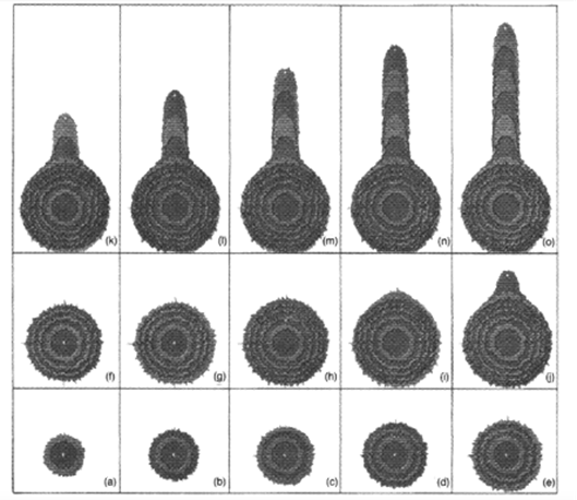
Figure 5: A computer simulation of spherical growth (a-h), and hypha extension growth (j-o). The position of the VSC is indicated by the white dot (Prosser, 1995).

N is how fast the vesicles are produced, and the ratio V/N represents how far is the VSC from the tip wall. In this equation, there is only one parameter. Therefore, this model implies that the shape of the hyphal tip is defined by a single parameter, which makes the VSC model simple and easy to apply under limited given conditions. However, this is also a deficiency of this model. There are other variabilities like the angle from the origin as the materials are incorporated in the cell wall, and the VSC could have some distance from the hyphal tip. Thus, the model is not sufficient when more details are given in the experiments, and more complex models that involve more parameters are needed (Prosser, 1995).

Growth of mycelium

Models at a higher level for fungal growth are built on lower-level models and would utilize basic information or omit some parameters that do not have influence to better describe the growth of aquatic fungi.

There is a relationship between the branching of mycelium and the macroscopic growth of fungi. The symmetric branching model to describe them is proposed by Viniegra-Gonzalez et al.. It first considers an interbranch mycelium network to have an average length of segments L_avshown in Equation 13:

$L_{\text{av}} = \frac{L_t}{N_s}$

Equation 13: The equation for the average length of segments of mycelium by Viniegra-Gonzalez et al. (Prosser, 1995).

L_t is the total length of hyphae and N_s is the segment number. N_s is also equal to 2(N_t-1) where N_t is the total number of tips. The model also takes the branching level k into consideration, which relates to specific mycelium growth rate u_x equation 14 below:

$\mu_x = \frac{(2 \ln 2) \overline{\mu_r}}{\overline{\gamma} L_{\text{av}}}$

Where

$\overline{\gamma} = \frac{2^{\overline{k} + 1} - 1}{2^{\overline{k}}}$

Equation 14: The equation for the growth rate of mycelium (top) is linked to the branching level (bottom), k (Prosser, 1995).

Therefore, the model describes a relationship between the branching levels of mycelium and the mycelium growth rate, which is also the hyphal extension rate. This model has a good fit with experimental data from the growth of fungi G. candidum. This model is also macroscopic since it predicts the observed difference in the mycelium population and fungi growth, thus, it provides a valuable approach for image techniques for analysis (Prosser, 1995).

Conclusion

This essay focuses on mathematical models that can describe many of the behaviours of aquatic fungi, including population growth, leaf decomposition, bioremediation, parasitism, and growth of the physical fungal body.

It is important to consider factors like temperature, pH, and nutrient availability when creating a mathematical model for behaviors of an organism. When creating a mathematical model, no information should be omitted as this may result in a model that does not accurately predict the desired behavior. Of course, no model can perfectly encapsulate the behaviors of a living organism. In this essay, ways of using the logistical model to monitor aquatic fungi populations were described. With this model, researchers can analyze how environmental changes impact aquatic fungi populations.

Moreover, models describing how parasitic aquatic fungi impact frog populations were introduced. By monitoring their spread (looking at factors that can inhibit and enhance their spread), these models can hopefully mitigate the negative effects that aquatic fungi have on frog species. It was found that Batrachochytrium Dendrobatidis reproduced best in warm climates, at temperatures below 28 °C, since anything above 32 °C was deadly to the fungus. Additionally, despite all the design solutions chytrids possess to aid in fungal proliferation and spore dispersal, Bd was weak to violacein, a fungicide produced by Janthinobacteriumlividum. This design solution that some frogs employ was sufficient to prevent the local extermination of frog species by chytridiomycosis.

Furthermore, aquatic fungi are invaluable when it comes to the breakdown of plant litter in aquatic ecosystems. Models relating fungi colonization and substrate weight have been described in this paper. Fungal biomass can also be modeled using an equation indicating how much space there is on a substrate for fungi to attach. The more space available, the larger the biomass. Aquatic fungi work cleverly to use every bit of their resources. This design solution is seen in Equation 6, which shows how they use every bit of substrate they can attach to, to gain access to the most nutrients. Models describing how fungal biomass grows during decomposition can provide insight into what aquatic fungi gain from this interaction.

Also, aquatic fungi possessed the ability to perform bioremediation. Knowing how to quantify aquatic fungi's contributions in removing pollutants from water can encourage its widespread use in bioremediation. The model included in this paper uses differential equations to describe the rate at which aquatic fungi can remove pollutants, specifically dyes, from water. The model is another example of the design solution mentioned above: fungi will use every bit of the resource available to them, so as to not exert unnecessary energy in looking for more nutrients when they have an abundance of them available, whether that is in naturally occurring substrates, or pollutants.

Additionally, models explaining hyphal growth were provided, shining a light on how fungi are able to grow the network that provides them with nutrients. Equations describing mycelial growth were also provided, including their branching patterns. The shape of the fungal tip and the branching level of the mycelium both play a role in fungal growth, and these models provide insight into how fungi grow to strategically maximize the mycelium surface area to absorb nutrients for their survival. In sum, models to describe fungal growth – in the context of population, parasitism, decomposition, bioremediation, and structure – can provide valuable insight into the beautiful patterns and behaviors seen in aquatic fungi.

References

Ackleh, A. S., Carter, J., Chellamuthu, V. K., & Ma, B. (2016). A model for the interaction of frog population dynamics with Batrachochytrium dendrobatidis, Janthinobacterium lividum and temperature and its implication for chytridiomycosis management. Ecological Modelling, 320, 158-169. https://doi.org/https://doi.org/10.1016/j.ecolmodel.2015.09.015

Allman, E. S., & Rhodes, J. A. (2004). Mathematical models in biology: an introduction. Cambridge University Press. http://catdir.loc.gov/catdir/samples/cam041/2003043929.html

Bärlocher, F. (1980). Leaf-eating invertebrates as competitors of aquatic hyphomycetes. Oecologia, 47, 303-306.

Briggs, C. J., Knapp, R. A., & Vredenburg, V. T. (2010). Enzootic and epizootic dynamics of the chytrid fungal pathogen of amphibians. Proceedings of the National Academy of Sciences, 107(21), 9695-9700. https://doi.org/doi:10.1073/pnas.0912886107

Cornish-Bowden, A. (2015). One hundred years of Michaelis–Menten kinetics. Perspectives in Science, 4, 3-9. https://doi.org/https://doi.org/10.1016/j.pisc.2014.12.002

Dantigny, P. (2021). Applications of predictive modeling techniques to fungal growth in foods. Current Opinion in Food Science, 38, 86-90. https://doi.org/https://doi.org/10.1016/j.cofs.2020.10.028

Dym, C. L. (2004). Principles of mathematical modeling (Second edition. ed.). Elsevier Academic Press. http://www.123library.org/book_details/?id=38577

Falconer, R. E., Bown, J. L., McAdam, E., Perez-Reche, P., Sampson, A. T., van den Bulcke, J., & White, N. A. (2010). Modelling fungal colonies and communities: challenges and opportunities. IMA Fungus, 1(2), 155-159. https://doi.org/10.5598/imafungus.2010.01.02.07

Goyal, A., Sanghi, R., Misra, A. K., & Shukla, J. B. (2014). Modeling and analysis of the removal of an organic pollutant from a water body using fungi. Applied Mathematical Modelling, 38(19), 4863-4871. https://doi.org/https://doi.org/10.1016/j.apm.2014.03.050

Harer, K. M. (2014). A mathematical model of the spread of Batrachochytrium dendrobatidis in the Cascades frog (Rana cascadae) [Masters Thesis, California State Polytechnic University, Humboldt]. ScholarWorks. http://www.engineeringvillage.com/controller/servlet/OpenURL?genre=book&isbn=9780122265518

Krauss, G.-J., Solé, M., Krauss, G., Schlosser, D., Wesenberg, D., & Bärlocher, F. (2011). Fungi in freshwaters: ecology, physiology and biochemical potential. FEMS Microbiology Reviews, 35(4), 620-651. https://doi.org/10.1111/j.1574-6976.2011.00266.x

Künzler, M. (2018). How fungi defend themselves against microbial competitors and animal predators. PLoS Pathog, 14(9), e1007184. https://doi.org/10.1371/journal.ppat.1007184

Prosser, J. I. (1995). Kinetics of Filamentous Growth and Branching. In N. A. R. Gow & G. M. Gadd (Eds.), The Growing Fungus (pp. 301-318). Springer Netherlands. https://doi.org/10.1007/978-0-585-27576-5_14

Shi, T., & Wang, H. (2022). Mathematical Modeling Analysis and Optimization of Fungal Diversity Growth. https://doi.org/10.48550/arXiv.2208.02564

Thacharodi, A., Hassan, S., Singh, T., Mandal, R., Khan, H. A., Hussain, M. A., & Pugazhendhi, A. (2023). Bioremediation of polycyclic aromatic hydrocarbons: An updated microbiological review. Chemosphere, 138498.

Vass, M., Eriksson, K., Carlsson-Graner, U., Wikner, J., & Andersson, A. (2022). Co-occurrences enhance our understanding of aquatic fungal metacommunity assembly and reveal potential host–parasite interactions. FEMS Microbiology Ecology, 98(11). https://doi.org/10.1093/femsec/fiac120