Just Keep Swimming: Structure, Movement, and Light Interactions of Unicellular Green Algae

A Mathematical Approach to Understanding Volvox

An Investigation into the Mathematical Modeling of the Properties of Gonium

Andrew D’Argenio, Breanna D’Ettorre, Lucas Elliott, and Joseph Gad

ABSTRACT

The multicellular algae of genus Gonium have been shown to be a remarkable feat of evolution. It can be difficult to fully appreciate the colonial algae’s ingenuity when only observing the organism. By attempting to model their behaviour, insight into the beauty of their design can be gained in the most universal language, math. Through the modelling of Gonium’s flagellar fluid dynamics, we can see just how important the asymmetrical forces produced by the peripheral flagella is the colony’s reorientation mechanism. The absence of this imbalance of forces will leave the colony without their unique wavy trajectory that allows them to better scan their environment during phototaxis. This evolutionary advantage is only possible due to the organism multicellularity, which when analyzed mathematically in comparison to unicellular populations we see the emergence of another advantage, the reduction of accident rates. Interestingly, Gonium can even be used as a biofuel as it has a reasonable ability to sequester carbon dioxide and provide energy through photosynthesis, thus, demonstrating a potential to be used as an environmentally friendly biofuel. The details of Gonium’s chemical pathways and how they contribute to the formation of the extracellular matrix can be understood using computational linguistics. To best understand Gonium’s evolutionary advantages through a mathematical lens, we will first model the fluid dynamics of the flagella of a colony, then analyze the benefits of multicellularity through mathematical simulation. We then change course and quantify Gonium’s ability as a biofuel before concluding with an analysis of Gonium as algae system using formal language theory.

INTRODUCTION

Math is a language beyond all words that we have created. It exists in every object, in every scale that one could imagine, and describes everything that could possibly be realized-—even Gonium, the magnificent sixteen-celled algae. The mathematical design of Gonium has been developed over thousands of years of evolution, culminating in a microalgae with all the necessary adaptations for its environment.

Gonium’s multiple biflagellate cells that are enveloped within a gelatinous matrix vary in number depending on the species. Colonies can contain 4, 8, 16, or 32 cells of the same size organized in a flat plate. These phototrophic organisms rely on phototaxis to orient themselves to perform photosynthesis. The flagellar movement of the multicellular organism allows it to orient its eyespot in the direction of the light.

Gonium’s morphology and behavior exhibit significant mathematical relationships that can be modeled through computational geometry. Beyond the simple behavior and environmental interactions of Gonium, it has been discovered that for the evolution of Gonium, the motivation behind evolution can be mathematically modeled, and results from a reduction of accident rates compared to single celled algae in the Gonium family like Chlamydomonas. On a large scale, the thermodynamic interactions of entire colonies of Gonium can be mathematically modeled and have been presented within the context of algal biofuel production. On a more theoretical level, Gonium can be examined through formal language theory, a mathematical and computer science-based theory that describes Gonium in terms of a system with inputs and outputs, which can be extended to understand why Gonium colonies have the specific extracellular matrix conformation they exhibit.

In the pages that follow, a story that follows the relationship between Gonium and the natural laws of math that govern this world will be woven, while the interactions between the two are examined and the forces governing its biology are unmasked. By exploring mathematics in Gonium, a connection between nature and design can be established in its purest form.

MODELLING THE FLUID DYNAMICS OF GONIUM FLAGELLA

Gonium’s helical swimming path is a result of the asymmetrical forces exerted by the outer cells. These forces result in a net torque on the colony that causing it to rotate about itself (Leptos et al., 2023). This process as described in more detail in the previous article titled An Investigation of the Physical properties of Gonium under the Phototaxis subsection. In the following section, this understanding will be expanded by modelling the fluid dynamics of the microorganism.

Gonium pectorale’s swimming, due to its small size of 40 μm and swimming speed of 40 μm/s, its Reynolds number is on the order of magnitude of 10^-3. These factors indicate that the colony’s swimming is ruled by Stokes equation (Lauga & Powers, 2009).

De Maldeprade’s fluid dynamical and computational model of the 16-celled organism’s swimming is based on the colony being described as thick disk. The disk’s axis of symmetry is $\hat{e}_3$ , as seen in Figure 1, and the colony’s averaged radius is α. The flagella, which significantly contribute to the friction of the colony, as such the must also be considered in the model. Thus, an effective radius of R must be considered, which extends from the center of the colony to the end of the flagella.

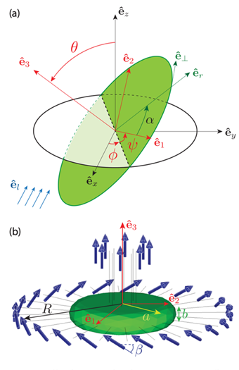
Figure 1: The details on the computational geometry of Gonium. (a) The coordinate systems and Euler angles where the lab frame is ( $\hat{e}_x, \hat{e}_y, \hat{e}_z$ ) and the frame attached to the colony is ( $\hat{e}_1, \hat{e}_2, \hat{e}_3$ ). $\hat{e}_3$ is the symmetry axis and ( $\hat{e}_1, \hat{e}_2$ ) is the plane of the body. The Euler angles ( $\theta, \phi, \psi$ ) connect the two frames: $\theta$ is the angle between $\hat{e}_3$ and $\hat{e}_z$ , $\phi$ the angle between $\hat{e}_x$ and the dotted line of nodes and $\psi$ the angle between the line of nodes and $\hat{e}_1$ . $\hat{e}_l = -\hat{e}_x$ is the direction of the incident light. (b) Gonium’s geometry for simulations. The green body (disk) has a radius a = 20 μm and a thickness b = 8 μm. The flagella (length 20 μm) are associated with a point force 20 μm from the cell body. The colony has an effective radius R, that extends from the center of the colony to the ends of the flagella. The 8 central flagella generate thrust while the 24 peripheral ones (tilted by β ≃ 30°) generate thrust and rotation (de Maleprade et al., 2020).

In the frame attached to the body of the colony, ( $\hat{e}_1, \hat{e}_2, \hat{e}_3$ ), the viscous force F_v and viscous torque L_v are related linearly to the colony’s velocity U and angular velocity Ω using the following equations:

$\mathbf{F}_v = -\eta R \begin{bmatrix}k_1 & 0 & 0 \0 & k_1 & 0 \0 & 0 & k_3\end{bmatrix} \mathbf{U}$

$  \mathbf{L}_v = -\eta R^3 \begin{bmatrix}l_1 & 0 & 0 \0 & l_1 & 0 \0 & 0 & l_3\end{bmatrix} \mathbf{\Omega}  $ .

Equation 1 and 2: The viscous force (F_v) and the viscous torque (L_v) of a Gonium colony. Where η is the viscosity of water, i.e., η = 1 mPa, the numbers k₁, k₃ are the translational and rotational friction along the transverse direction and l₁, l₃ are the translational and rotational friction along the axial direction. U is linear velocity and Ω is angular velocity (de Maleprade et al., 2020).

The angular velocity Ω can be expressed in the body frame, ( $\hat{e}_1, \hat{e}_2, \hat{e}_3$ ), using Euler’s angles ( $\theta, \phi, \psi$ ), illustrated in Figure 1,

$  \Omega = \begin{bmatrix}\dot{\theta} \cos \psi + \dot{\phi} \sin \theta \sin \psi \-\dot{\theta} \sin \psi + \dot{\phi} \sin \theta \cos \psi \\dot{\psi} + \dot{\phi} \cos \theta\end{bmatrix}  $ .

Equation 3: Angular velocity expressed in the body reference frame. Where ( $\theta, \phi, \psi$ ) are Euler’s angles, relating the colony’s frame to the lab frame (Symon, 1971).

The viscous forces F_v and torques L_v are balanced by the thrust and spin generated by the flagellar beating. The flagella from the center cells do not generate any torque, however they do create a net thrust of $F_c \hat{e}_3$ , as seen in Figure 1 (b). The outer flagella participate in both the propulsive thrust and the rotation of the colony. The net force and torque produced by all the flagella are expressed using the following equations:

$F = F_c \hat{e}_3 + \int_0^{2\pi} f_p \, d\alpha, \quad L = \int_0^{2\pi} \mathbf{R} \times f_p \, d\alpha$

Equations 4 and 5: The net force (F) and net torque (L) produced by the 32 flagella of a 16-celled Gonium colony. Where $f_p(\alpha)$ is the force produced by the peripheral flagella that is dependent on the angle α as seen in Figure 1 (a). R is the effective radius. F_c is the net force produced by the 4 center cells of the colony, exerted in the $\hat{e}_3$ direction (de Maleprade et al., 2020).

When a colony is not experiencing phototactic cues, the peripheral cells of a perfectly symmetrical Gonium would produce a force fp that has no angle α dependence, resulting in a force and torque that is purely axial.

$\mathbf{F}^{(0)} = [F_c + 2\pi f_{p\parallel}^{(0)}] \hat{e}3, \quad \mathbf{L}^{(0)} = 2\pi R f{p\perp}^{(0)} \hat{e}_3.$ .

Equations 6 and 7: The net force ( $\mathbf{F}^{(0)}$ ) and torque ( $\mathbf{L}^{(0)}$ ) of a colony with no angle dependence, i.e. α=0. Where $f_{p\parallel}$ is the component of the force produced by the peripheral flagella that is parallel to the colony and $f_{p\perp}$ is the component that is perpendicular to the colony (de Maleprade et al., 2020).

This organism has a straight swimming path due to the axial net force and torque along $\hat{e}_3$ . Since we know that Gonium has helical trajectories, this suggests that the forces produced by the peripheral flagella f_p are not symmetrical. It is this imbalance in the distribution of forces that produce the nonzero components of the net force F and torque L that are perpendicular to $\hat{e}_3$ , which in turn deflects the colony’s trajectory resulting in the helical swimming path. The simplest equation of the imbalance that match Gonium’s helical trajectories is a modulation of the force created by the outer flagella is shown in equation 8.

$f_p(\alpha) = f_p^{(0)} (1 + \xi \cos \alpha)$ ,

Equation 8: The modulation of the force created by the peripheral flagella. Where the imbalance factor ξ is 0≤ ξ ≤1(de Maleprade et al., 2020).

According to this model, there is a stronger flagellar force along $\hat{e}_1$ and the net force and torque have components in the ( $\hat{e}_2$ , $\hat{e}_3$ ) plane. The combined effect of the transvers force and torque components is what allows Gonium to their overall swimming path despite having such an imbalance.

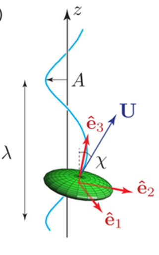
Figure 2: Helical trajectory of a Gonium colony while swimming. The colony (green ellipsoid) has a velocity U along a helical path (blue line). The oscillation has a wavelength λ, amplitude A, and pitch angle χ. The frame ( $\hat{e}_1, \hat{e}_2, \hat{e}_3$ ) is attached to the colony’s body (de Maleprade et al., 2020).

The pitch angle χ of Gonium’s helical trajectory still needs to be explained by the uneven distribution of forces. A colony that is swimming along the $\hat{e}_z$ axis, as shown in Figure 2 will have $\hat{e}_3$ form a cone about $\hat{e}_z$ where its apex angle will be a constant ζ. The angular velocity vector Ω will be along $\hat{e}_z$ . Using the Euler representation of Ω, this results in θ = ζ, ψ=0 and $\Omega = \dot{\phi} (\sin \zeta \hat{e}_2 + \cos \zeta \hat{e}_3)$ where the constant φ is negative. The pitch angle χ is the angle between U, the colony’s velocity, and $\hat{e}_z$ . Due to the resistance matrices having different values when measured in different directions and the axial force Fc produced by the center flagella, the pitch angle is greater than the apex angle ζ between $\hat{e}_3$ and $\hat{e}_z$ . This will cause lateral excursions, meaning the colony will move from side to side, while keeping its symmetry axis $\hat{e}_z$ nearly aligned with the average swimming direction $\hat{e}_z$ . With further expansion to the first order in the imbalance amplitude ξ, the force and torque balance is represented by equation 9.

$\tan \chi = \frac{\xi}{2} \left{ \frac{l_3}{l_1} \tan \beta + \frac{k_3}{k_1} \frac{1}{\tan \beta} \frac{1}{1 + \frac{F_c}{2\pi f_{p\parallel}^{(0)}}} \right}$

Equation 9: The relationship between the pitch angle (χ) and the imbalance amplitude (ξ). Where k1, k3 are the translational and rotational friction along the transverse direction and l1, l3 are the translational and rotational friction along the axial direction. β is the angle that the peripheral flagella have with the colony. F_c is the net force produced by the 4 center cells of the colony. $f_{p\parallel}$ is the component of the force produced by the peripheral flagella that is parallel to the colony (de Maleprade et al., 2020).

From this equation we can see that a colony without an asymmetrical force distribution ( $\xi = 0$ ) will have a straight swimming path (χ=0) (de Maleprade et al., 2020).

 Interestingly, this model further demonstrates the need for the asymmetrical force exertion by the flagella explain in our previous article. In the previous article the necessity of Gonium’s trajectory having a waviness character, shown in Figure 3, to its phototactic reorientation. Briefly, despite this factor coming at the cost of swimming efficiency, it benefits efficient reorientation as it increases the colony’s field of view allowing for a better perception of its environment so that it can better detect directions of light (de Maleprade et al., 2020). This mathematical model demonstrates the importance of the asymmetrical flagellar forces for the organism’s wide arcs during swimming. From this last equation, we can see that if the asymmetrical force distribution (ξ) is zero then the pitch angle (χ) of the colony’s swimming path will also be zero. This demonstrates that without the force asymmetry Gonium would not be able to swim with these wide arcs, negatively impacting the colony’s reorientation mechanism. This only further demonstrates the effectiveness of the organism’s flagellar design at ensuring direct and efficient phototactic reorientation.

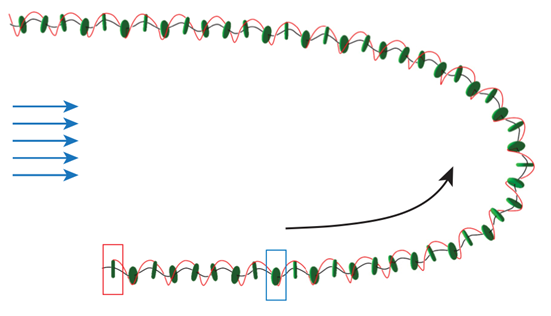
Figure 3: Wavy trajectory of Gonium during reorientation. Its initial position is marked by the red rectangle. When the colony reaches the blue rectangle, a light is switched on from the left (blue arrows). The black line shows the trajectory, and the red line shows the rotation of the body by following the position of the maximal force, α = 0 (de Maleprade et al., 2020).

MATHEMATICAL MODELING OF GONIUM BIOFUEL VIABILITY

Algae have long been researched in biofuels for their unique ability to sequester CO₂ and provide bioenergy through photosynthesis and organic matter processing. Rapidly growing algal biofuels, while not yet highly scalable, hold the potential to be a renewable energy source with a significantly lower carbon footprint and environmental impact than fossil fuel-based energy. According to Hannon et al., nuclear transformation of the algae of choice must be possible to maximize the production of biofuels. This puts Gonium in a position of interest, as it is one of not very many algae from the Chlorophyceae family that has been successfully edited (Lerche and Hallmann, 2009). While it may not be the ideal choice for algal biofuels, it can be proven with mathematical modeling that it may be a great addition, and at the very least, the research done on Gonium can provide valuable conclusions for future research into other algal species.

 A recent study in 2022 provided an intriguing mathematical model that assesses the efficiency of CO₂ fixation and biomass growth for Gonium pectorale, one of the most common and well-researched species of Gonium. One of the most effective methods of creating fuels from algae colonies is called pyrolysis, which refers to the heating of an organic material in an environment without oxygen. Pyrolysis may happen as simply as a cook caramelizing onions, or as intricately as a machine synthesizing and treating oils. When dry, algae material like Gonium is pyrolyzed, then pyrolysis oil, syngas, and bio-char are all produced (Demirbas & Arin, 2002). Pyrolysis oil is a type of bio-oil, that functions similarly to conventional oil after processing. Syngas is a mixture of carbon monoxide and hydrogen that can be used for fuel. Bio-char is similar to charcoal. Conveniently, all of these products of pyrolysis can be used for energy production, and the energy from just the syngas yield is enough to fuel the reaction multiple times over. A simple illustration of the pyrolysis reaction for biofuel production can be seen in Figure 4.

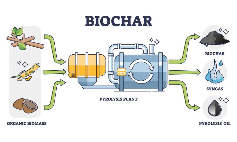
Figure 4: Pyrolysis-Based Biofuel Production. Dried biomass is input and heated in the absence of oxygen, producing a yield of biochar, syngas, and pyrolysis oil (“Pyrolysis”, 2022).

 To utilize pyrolysis oil production in the most ecologically positive way, Altriki asks readers to consider the use of Gonium. Microalgae take significantly less space than other organic matter, can be farmed with wastewater, and have a relatively high yield rate from pyrolysis (Altriki et al., 2022; Demirbas & Arin, 2002). To determine the pyrolytic efficiency of Gonium, researchers had to use thermogravimetric (TG) analysis and mathematical modeling to find the activation energy of the pyrolysis of Gonium. Thermogravimetric analysis involves consistently measuring the mass of a sample over a period of time during which the temperature is increased slowly and incrementally. This is an important value as it allows researchers to determine the amount of energy required to breach the activation energy barrier of different steps of pyrolysis, which might include pyrolysis of proteins, carbohydrates, and fats present in Gonium. A simple mathematical model can be used to determine the activation energy from this TG value. The activation energy (E_a) of a reaction can be determined at any conversion rate by the slope of the graph of y = $\ln\left(\frac{d\alpha}{dt}\right)$ ) plotted against 1/T, in something called an Arrhenius Plot. An example of this graph can be seen in Figure 5. In simpler words, this is the plot of the natural log of the rate of change of the degree of conversion, plotted inversely against temperature.

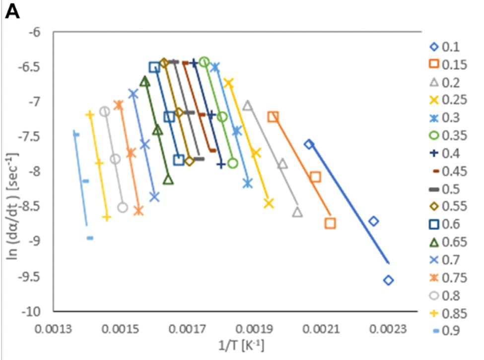
Figure 5: Arrhenius Plots of G. Pectorale at various conversion rates. Conversion rates are an indicator of how far along the pyrolysis reaction of Gonium is, ranging from .1 to .9 completed, or 10% to 90% completed (Altriki et al., 2022).

The slopes of these plots can be calculated to determine the exact activation energies at these conversion rates against the inverse of temperature in Kelvin, where is the conversion rate, and be calculated easily with the equation:

$\alpha = \frac{\omega_0 - \omega}{\omega_0 - \omega_f}$

Equation 10: Degree of Conversion: In this equation, w₀ is the initial mass of the sample, w_f is the final mass, and w is the mass at the time of measurement.

The value of α can be measured easily with TG analysis, especially in a curve like the one in Figure 6. The outcome is the ability to determine the degree of conversion of our algal sample at any point of temperature, which in turn is important to the modeling process that allows for the derivation of activation energy.

Figure 6: TG Analysis of Gonium at different temperatures. α can be easily found through using the weight percentage values in the equation for the degree of conversion, and this TG plot gives the important weight percentage values for this use (Altriki et al., 2022).

 After calculating the value of activation energy from the slopes of our Arrhenius plots, that value can be utilized in thermodynamic Equations 11 and 12. The Gibbs free energy and enthalpy of the reaction give a better perspective of the overall trends of the reaction, and how much energy is produced.

$\Delta H = E_a - RT$

$\Delta G = E_a + R T_p \ln \left( \frac{K_B T_p}{hA} \right)$

Equations 11 and 12: Enthalpy of Reaction and Gibbs Free Energy. Here, R is the gas constant, T_p is the maximum rate of change of the degree of conversion reached in TG analysis, K_B is the Boltzmanns constant, h is Planck’s constant, and A is the preexponential factor, calculated from the Arrenhuis plots (Altriki et al., 2022).

In these equations, H is the amount of energy required to be put into the reaction from our starting temperature. More importantly, G denotes the total change in energy of the system, which allows the visualization of the efficiency in energy created from this reaction. One average calculated from the process found a G of 176-214 kj/mol, notably above “the values of waste red peppers (139.0 kJ/mol) and rice straw (165.1 kJ/mol)” (Altriki et al., 2022). In this way, Gonium presents as an efficient fuel source compared to some existing sources! In addition to providing reliable fuel capabilities, Gonium also has the ability to sequester carbon in the process.

 Gonium’s sequestration of carbon follows a simpler equation similar to most algae, calculated in 2016 to be:

CO₂ Biofixation = $\frac{\text{CPMCO}}{\text{MC}}$

Equation 13: CO₂ Biofixation in Algae. C is carbon content of the algae, P is productivity, or growth of the algae per day in g/L, MCO₂ is the molar mass of carbon dioxide and MC is the molar mass of carbon (Adamczyk et al., 2016).

Gonium’s maximum sequestration of carbon in ideal conditions of a 2 %CO₂ matrix returned a value of about 0.13 g/L/day, with an average productivity of 79 mg/L/day (Altriki et al., 2022). On a large scale, Gonium has reasonable efficiency in carbon sequestration, proving that Gonium could be used as an environmentally positive biofuel.

ANALYZING GONIUM WITH FORMAL LANGUAGE THEORY

Formal language theory was created by Noam Chomsky in the 1950s, building upon previous linguistic theories (Jäger & Rogers, 2012). Linguistic theories are not used only to understand languages, in fact, they are actually quite mathematical. They are fundamental in computer science but could be used to understand biological systems. To understand how formal language theory can be used to understand the way in which multicellular algae, such as Gonium, the basics of the theory must first be established.

In formal language theory, an alphabet is a finite set of symbols (Yoshida et al., 2005), just as 26 letters compose the English alphabet. These symbols can be arranged in different ways to make strings. If we extend the previous analogy, strings are equivalent to words in spoken languages. Formal languages involve a finite number of strings, which make up a finite vocabulary (Jäger & Rogers, 2012). This vocabulary is analogous to a spoken language’s vocabulary i.e., a set of words. Vocabulary will be denoted by the symbol Σ (Jäger & Rogers, 2012).

With that being said, grammar consists of a vocabulary Σ, as well as three other elements, R, NT, and S (Jäger & Rogers, 2012). R represents the set of rules that exist in the language. Rules have a form that resembles the following:

$\alpha \rightarrow \beta \quad (14)$

This rule means that a string α is to be replaced with another string β. The rule could also be applied to larger strings in which α is embedded, as shown in the following example in which rule (14) is applied.

$\text{abcd}\alpha \rightarrow \text{abcd}\beta \quad (15)$

Another way of looking at the rules in formal language theory is as a set of relationships between inputs and outputs. This idea can be extended to biological systems, and chemical reactions that occur within them (Jäger & Rogers, 2012). In the previous essay, the oxidation of monolignols catalyzed by Gonium’s laccase enzymes as part of Gonium’s ability to produce depolluting enzymes was discussed (Solomon et al., 1996). This reaction can be modelled using formal language theory. If m is a string representing monolignol, and p is a string representing lignin polymer, the product of the metabolic pathway, the following rule can be used to represent the reaction.

m→ p

(16)

When m is input into Gonium, the rule dictates that it will be replaced by p. Of course, this is a simplification of a more complex reaction mechanism, which has intermediate products. This is where the notion of non-terminals, denoted by NT, and terminals come into play (Jäger & Rogers, 2012). Terminals are the strings produced after a series of rules have been applied, or in other words, the end product. These terminal strings are what make up the vocabulary Σ previously discussed. NT, which stands for non-terminal, on the other hand, are the precursors to the terminal strings. They are never the final terminal. The last element that makes up grammar is S, which stands for start, which is the string that the rules first apply to and from which a series of modifications is initiated. S is a member of the NT set, seeing that it is the first precursor of all the terminal strings.

If we return to the previous example regarding Gonium’s lactase enzymes and the reaction it catalyzes, we see that monolignol would be the starting non-terminal string, the intermediate products would also be non-terminals, and the final product of the metabolic pathway, lignin polymer, would be a terminal string. Each step of the reaction would be represented as a rule, transforming one string into another.

If all of Gonium’s chemical reactions were to be modeled using formal language theory, the cell could be modeled as a system of rewriting rules in a matrix as such (Yoshida et al., 2005):

$(A_1 \rightarrow \omega_1, A_2 \rightarrow \omega_2, \ldots, A_k \rightarrow \omega_k) \quad (17)$

This means that for every chemical in the set of A₁ to A_kreceived by the organism, the corresponding chemical in the set of ω₁ to ω_k is output. Each of these rules can be modeled as their own independent system, which will be referred to as a “pseudo cell” (Yoshida et al., 2005). Pseudo cells make up one algal cell, and the system of algal cells make up the Gonium colony.

The system that makes up a Gonium colony, as defined by formal language theory, is the following (Yoshida et al., 2005):

$\Pi = (NT, \Sigma, \Lambda, M, s, R_1, R_2, \ldots, R_m, S) \quad (18)$

The N, T, and S in (18) are the same that were previously defined. Λ represents the set in which the pseudo cells are numbered or, in other words, the set in which the individual reactions occurring in the cells are numbered. R₁ through R_m represents the rule associated with each pseudo cell, with m being the number of pseudo cells (Yoshida et al., 2005). The only values left to define are M and s (not to be confused with S). These values together make up the “algae structure” (Yoshida et al., 2005). M consists of sets of pseudo cells that “‘cooperate’ with one another” (Yoshida et al., 2005), as would be the case for reactions that are closely related or are part of the same pathway. The symbol s represents the existence of a membrane that encloses the cells. It is a binary value. If s equals 1, the membrane is present. If s equals 0, there is no membrane present.

As can be seen in Figure 7, adapted from Proyecto Agua (2018), Gonium’s 16 cells are not tightly packed. Rather, there is space between the cells. There is no membrane isolating the Gonium colony from the fluid surrounding it, which would mean that the formal language theory representation of Gonium would have s as 0.

Therefore, (18) can be rewritten in the following way, with the subscript G representing Gonium (Yoshida et al., 2005):

$\Pi_G = (NT, \Sigma, \Lambda, M, 0, R_1, R_2, \ldots, R_m, S) \quad (19)$

Moreover, M was found to be a set in which the pseudo cells are all independent of each other, and do not cooperate. This can be represented visually in Figure 8, adapted from Yoshida et al. (2005).

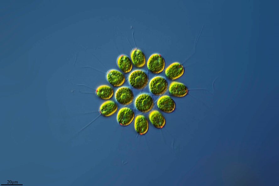
Figure 7: 16-cell colony of Gonium pectorale colony, pictured in lake water. The cells have spaces between them which make them open to the surrounding fluid environment (Proyecto Agua, 2018).

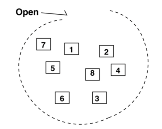
Figure 8: Visual representation of Gonium’s algae structure. There is no closed membrane surrounding the pseudo cells, numbered 1-8, which are all independent of each other (Yoshida et al., 2005).

Essentially, because of the isolation of each of the pseudo cells, and the lack of a surrounding membrane, formal language theory suggests that Gonium is limited in terms of the strings it can generate, or chemicals it can output (Yoshida et al., 2005). Formal language theory provides insight into how Gonium is structured. Having established the previous characteristics regarding Gonium’s structure, it is clear why Gonium’s extracellular matrix is more primitive than that of other organisms, such as Volvox, which exhibits both a membrane and cooperation between its pseudo cells when modeled using the techniques previously described. Gonium’s extracellular matrix composition is bound to be more limited than that of Volvox, which can form more complex strings, according to formal language theory, and thus has many more possible extracellular matrix compositions. This linguistic theory can also be used to model Gonium’s chemical processes and how different components in an algae system interact to accomplish Gonium’s biological goals.

MODELLING THE GROWTH OF GONIUM POPULATIONS: THE BENEFITS OF MULTICELLULARITY

Another set of significant adaptations that Gonium has evolved is of its most fundamental features, namely its multicellularity and its reproduction rate. The significance of these characteristics can be illustrated mathematically with the help of Gonium’s phylogenetic link to its more basal volvocine relative, Chlamydomonas. Indeed, in 1976, Walker and Williams were able to use mathematical models to highlight how the multicellular nature of this green algae mitigates some of the obstacles that its unicellular ancestor faces.

Among these, one of the most notable set of obstacles is referred to as the “accident rate”. It is the rate at which adverse events occur within a population of organisms of a certain species, causing the size of the population to diminish. These adverse events include the emigration or death through disease, predation, or competition of an organism.

The model adopted by the authors to study the accident rates and sizes corresponding to populations of Chlamydomonas and Gonium is a sequential representation of these quantities that relies on an assumption: Successive generations of Gonium and Chlamydomonas populations are separate, synchronous, and of constant duration. (This excludes situations where Gonium colonies exhibit accelerated reproduction due to mutilation or separation of their cells.)

Additionally, all colonies of Gonium are assimilated to the 4-celled species Gonium sacculiferum or Gonium sociale. Since each cell of a given colony is known to be individually viable (Swilley, 2018), each one is considered equivalent in its consumption of resources to an individual organism.

Finally, the rate of reproduction of 4-celled Gonium colonies and Chlamydomonas cells is described with respect to generational gaps. The duration of a generation of such Gonium colonies is considered equivalent to the duration of two generations of Chlamydomonas. Although not entirely accurate, this is logically coherent as, while Chlamydomonas cells only divide once into two daughter cells, each Gonium cell reproduces either sexually or asexually, producing a new colony, with sexual reproduction being slightly slower than its counterpart (Umen & Olson, 2012).

Considering the previous suppositions, the number of Chlamydomonas cells in the (2n+1)th generation of a population of such organisms is:

$\lambda_{2n+1} = 2(1 - \alpha_{2n})\lambda_{2n} \quad (20)$

where ${\lambda_k}_{k \in \mathbb{N}}$ is the number of cells in the kth generation and ${\alpha_k}_{k \in \mathbb{N}}$ is the accident rate (ratio of the number of deaths, emigrations, etc. to the number of individuals in the population) between the kth and (k+1)th generations of Chlamydomonas. This implies that the number of Chlamydomonas cells in the (2n+2)th generation is:

$\lambda_{2n+2} = 2(1 - \alpha_{2n+1}) \lambda_{2n+1} = 4(1 - \alpha_{2n})(1 - \alpha_{2n+1}) \lambda_{2n} \quad (21)$

Similarly, the number of Gonium colonies in the (2n+2)th generation of a population of Gonium is:

$\mu_{2n+2} = 4(1 - \beta_{2n})\mu_{2n} \quad (22)$

where ${\mu_k}_{k \in \mathbb{N}}$ is the number of cells in the kth generation and ${\beta_k}_{k \in \mathbb{N}}$ is the accident rate between the kth and (k+1)th generations of Gonium.

 After establishing these expressions, the authors study the development of populations of Gonium and Chlamydomonas as it relates to two variables. These two variables each correspond to distinct models (models A and B).

Model A: Development of populations of Gonium and Chlamydomonas as it relates to varying accident rates.

The first angle under which population development is studied (Model A) relies on the assumption that the accident rates ${\alpha_k}_{k \in \mathbb{N}}$ and ${\beta_k}_{k \in \mathbb{N}}$ can vary between generations and that the total number of Gonium and Chlamydomonas cells remains constant and equal to the carrying capacity N of the environment shared by the two populations. In this case we have, for any kth generation of the populations:

$\lambda_k + 4\mu_k = N \quad (23)$

Under these conditions, it can be shown that the population of Gonium will tend to overtake and replace that of Chlamydomonas. This trend is illustrated for N = 1000 individuals in Fig. 9, where Gonium replaces Chlamydomonas after 54 Chlamydomonas generations.

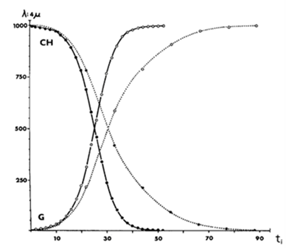
Figure 9: Replacement of Chlamydomonas population by Gonium during sexual reproduction (dotted lines) and asexual reproduction (solid lines). In an environment with carrying capacity N = 1000 individuals (i.e. Chlamydomonas or Gonium cells), where t_i represents the time corresponding to generation i. At t₀, we have $\lambda_0 = 1000 - 4\mu_0 = 9996$ and μ₀ = 1 (Walker & Williams, 1976).

Model B: development of populations of Gonium and Chlamydomonas as it relates to varying total size of populations.

The second pattern of development (Model B) assumes the accident rates α_k = α and β_k = β to be constant and that the total number of Gonium and Chlamydomonas cells is less than or equal to the carrying capacity N of their environment. We therefore have:

$\lambda_k + 4\mu_k \leq N \quad (24)$

Under these circumstances as with Model A, the population sizes can be described by the following expressions:

$\lambda_{2n} = \left(2(1 - \alpha)\right)^{2n} \lambda_0 \quad (25)$

$\mu_{2n} = \left(2(1 - \beta)\right)^{2n} \mu_0 \quad (26)$

where μ₀ = 1 and λ₀ ≤ 1 – μ₀, in which case it can again be shown that Gonium will replace Chlamydomonas at a generation n_a. n_a is demonstrated to be the smallest positive integer that satisfies:

$n_a \geq \frac{\log N - 2 \log 2}{\log (1 - \beta)} + 2 \log 2 \quad (27)$

This sequential analysis of Gonium serves to highlight the benefits of its multicellularity and the reproductive rate that it entails. Indeed, as suggested by these models, this multicellular nature must have been a key element in allowing Gonium’s survival and rapid multiplication in an environment populated by organisms like its ancestor, Chlamydomonas, with which Gonium would need to compete for the various resources that allow for its survival.

CONCLUSION

After diving deeper into the mathematical world of Gonium, understanding the complex interconnectedness of math throughout every aspect of Gonium becomes simpler. Evolution, as the world’s greatest designer, has demonstrated all of the mathematical processes described here and much more, to a degree that human’s mathematical systems have yet to reach. Just the mathematical development that had to take place for Gonium to be able to achieve helical propulsion through flagellar forces is enough to give any college student a headache, as one might know. The driving force of evolution becomes much more mathematically complex upon the consideration of how it branches out across genetic trees, and how much the math in Chlamydomonas or Volvox differs from that of Gonium.

 From the evolution of Chlamydomonas to Gonium, the emerging derived genus faced many conundrums, but mathematics served to direct evolutionary responses that allowed Gonium to overcome them. When Gonium needed to survive in its specific, low Reynolds-number environment through the movement and positioning for the gathering of light, it’s no wonder that it developed an ideal geometric structure to allow for helical propulsion patterns that contribute to light activation across all cells. Even more so, the advanced interactions between the flagella of the sixteen individual cells culminate perfectly in a wavy trajectory, maximizing its ability to search for light through the mathematical balancing of numerous unequal forces.

 When faced with the deadly hand of accident rates in single cellular organisms, the evolution to multicellularity in Gonium itself is a valuable design solution that intrinsically weighs the probabilities of success and failure, and votes in favor of the stable, robust Gonium.

The utilization of formal language theory has provided insight into the limitations set on Gonium and its ability to create different compositions of its extracellular matrix. This information explains why Gonium is configured in the way that it is. In other words, Gonium’s configuration can be seen as a design solution; it is the best Gonium could do with its limited resources thanks to the lack of cooperation between pseudo cells. Formal language theory is a powerful tool which could be used to analyze other cellular components to better understand the way in which they work and what the limitations that are set upon them are.

It may seem at first that the utilization of Gonium for biofuels does not provide much of an insight into the natural design of Gonium, but if the reader steps back to view Gonium from a wider lens, it may become clearer. The consideration of Gonium for algal biofuels is only possible because of the numerous design solutions that Gonium has perfected. The increased efficiency in fuel compared to plant waste can be attributed to the incredibly efficient organism that Gonium has to be when it performs such a wide variety of complex behaviors in such a small package. Additionally, when the carbon fixation of Gonium is explored, it is important to remember the role of carbon consumption in Gonium’s only energy source. It is because Gonium survives solely on photosynthesis that it has developed systems capable of such efficient carbon fixation.

In this way, both the evaluation of Gonium as a biofuel and the evaluation of Gonium through formal language theory can be seen as a perspective lens through which the reader can connect to the design solutions of Gonium, the way that researchers have in formal mathematical analyses. This can be visualized clearly in Figure 10, which highlights mathematical design solutions within this essay and possible mathematical outlooks one can take on the aforementioned solutions.

As the story told by mathematics in Gonium comes to a close, all credit should be attributed to nature, in evolution, for doing all the math for little Gonium. Humans created mathematics to be a language that makes sense of the greater natural system that couldn’t be seen, which is something to keep in mind when analyzing natural systems using mathematics. Engineers should be able to push this mindset even further, taking inspiration from nature for the mathematical design of efficient systems. A perfect example is in algal biofuels, where Demirbas & Arin estimated in 2002 that utilizing algal biofuels will not only become quickly more efficient than fossil fuel-based systems, but exponentially more important, as we begin to understand exactly what an unrenewable resource means.

 To continue to develop more efficient and robust solutions to the problems faced today, engineers must focus not only on using synthetic mathematical systems to their fullest extent, but analyzing further the hidden math in nature, with efficiency that seems boundless in comparison. This idea contributes heavily to the increasing importance of hybrid design in our world and makes even an organism like Gonium much more significant than anyone could tell at first glance.

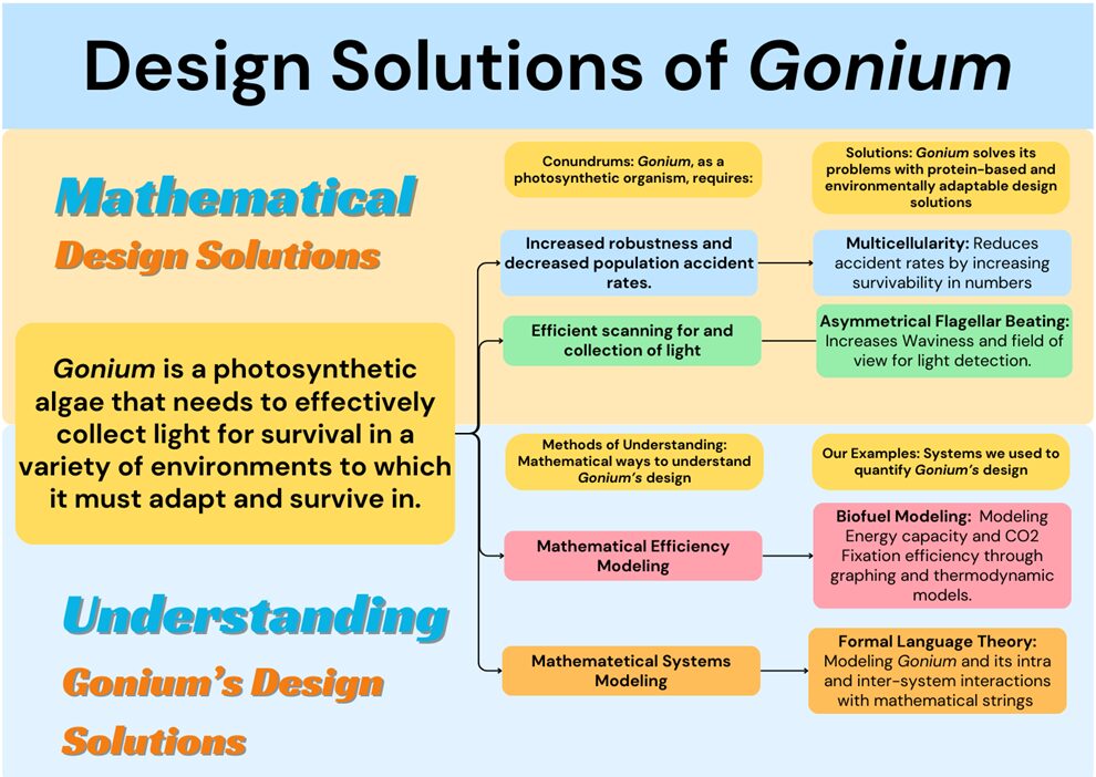
Figure 10: Design Solutions and Mathematical Perspectives of Gonium. This flowchart can be used to visualized conundrums and mathematical solutions within Gonium as well as the way that Gonium is evaluated mathematically in the scientific world.

REFERENCES

Adamczyk, M., Lasek, J., & Skawińska, A. (2016). CO2 Biofixation and Growth Kinetics of Chlorella vulgaris and Nannochloropsis gaditana. Applied Biochemistry and Biotechnology, 179(7), 1248-1261. https://doi.org/10.1007/s12010-016-2062-3

Altriki, A., Ali, I., Razzak, S. A., Ahmad, I., & Farooq, W. (2022). Assessment of CO2 biofixation and bioenergy potential of microalga Gonium pectorale through its biomass pyrolysis, and elucidation of pyrolysis reaction via kinetics modeling and artificial neural network. Frontiers in Bioengineering and Biotechnology, 10. https://doi.org/10.3389/fbioe.2022.925391

de Maleprade, H., Moisy, F., Ishikawa, T., & Goldstein, R. E. (2020). Motility and phototaxis of Gonium, the simplest differentiated colonial alga. Physical Review E, 101(2), 022416. https://doi.org/10.1103/PhysRevE.101.022416

Demirbas, A., & Arin, G. (2002). An Overview of Biomass Pyrolysis. Energy Sources, 24(5), 471-482. https://doi.org/10.1080/00908310252889979

Hannon, M., Gimpel, J., Tran, M., Rasala, B., & Mayfield, S. (2010). Biofuels from algae: challenges and potential. Biofuels, 1(5), 763-784. https://doi.org/10.4155/bfs.10.44

Hanschen, E. R., Marriage, T. N., Ferris, P. J., Hamaji, T., Toyoda, A., Fujiyama, A., Neme, R., Noguchi, H., Minakuchi, Y., Suzuki, M., Kawai-Toyooka, H., Smith, D. R., Sparks, H., Anderson, J., Bakarić, R., Luria, V., Karger, A., Kirschner, M. W., Durand, P. M., . . . Olson, B. J. S. C. (2016). The Gonium pectorale genome demonstrates co-option of cell cycle regulation during the evolution of multicellularity. Nature Communications, 7(1), 11370. https://doi.org/10.1038/ncomms11370

Hayama, M., Nakada, T., Hamaji, T., & Nozaki, H. (2010). Morphology, molecular phylogeny and taxonomy of Gonium maiaprilis sp. nov. (Goniaceae, Chlorophyta) from Japan. Phycologia, 49(3), 221-234. https://doi.org/10.2216/ph09-56.1

Jäger, G., & Rogers, J. (2012). Formal language theory: refining the Chomsky hierarchy. Philos Trans R Soc Lond B Biol Sci, 367(1598), 1956-1970. https://doi.org/10.1098/rstb.2012.0077

Lauga, E., & Powers, T. R. (2009). The hydrodynamics of swimming microorganisms. Reports on progress in physics, 72(9), 096601.

Leptos, K. C., Chioccioli, M., Furlan, S., Pesci, A. I., & Goldstein, R. E. (2023). Phototaxis of Chlamydomonas arises from a tuned adaptive photoresponse shared with multicellular Volvocine green algae. Phys Rev E, 107(1-1), 014404. https://doi.org/10.1103/PhysRevE.107.014404

Lerche, K., & Hallmann, A. (2009). Stable nuclear transformation of Gonium pectorale. BMC Biotechnology, 9(1), 64. https://doi.org/10.1186/1472-6750-9-64

Proyecto Agua. “Dieciséis Nudos Para Una Alfombra Mágica. Gonium Pectorale, Arroyo de Sogo.” Flickr, Yahoo!, 20 Oct. 2023, www.flickr.com/photos/microagua/27736037969/in/photostream/.

Pyrolysis: the future of hydrogen production | FASTECH. (2022, July 21). https://www.fastechus.com/blog/pyrolysis-the-future-of-hydrogen-production

Santhakumaran, P., Kookal, S. K., Mathew, L., & Ray, J. G. (2019). Bioprospecting of Three Rapid-Growing Freshwater Green Algae, Promising Biomass for Biodiesel Production. BioEnergy Research, 12(3), 680-693. https://doi.org/10.1007/s12155-019-09990-9

Solomon, E. I., Sundaram, U. M., & Machonkin, T. E. (1996). Multicopper Oxidases and Oxygenases. Chemical Reviews, 96(7), 2563–2606. https://doi.org/10.1021/cr950046o

Swilley, K. L. (2018). Phenotypic analysis of two unicellular Gonium pectorale mutants defective in extracellular matrix assembly. https://krex.k-state.edu/bitstream/handle/2097/38911/KaseySwilley2018.pdf?sequence=1&isAllowed=y

Symon, K. R. (1971). Mechanics (3d ed.). Addison-Wesley Pub. Co. http://www.gbv.de/dms/bowker/toc/9780201073928.pdf

Yoshida, H., Yokomori, T., & Suyama, A. (2005). A simple classification of the volvocine algae by formal languages. Bull Math Biol, 67(6), 1339-1354. https://doi.org/10.1016/j.bulm.2005.03.001

Related Articles

Other Articles

The Chemistry Lying Deep Within a Volvox Colony

Robinson Libman, Meryem Louni, Ryan McGibbon, and Ali Najjar

Abstract Despite their apparent simplicity as microorganisms, Volvox are extremely complex living systems whose secrets have yet to be fully uncovered. This paper dives deep within Volvox to tackle the key chemical phenomena responsible for the basic functioning of the

Read More »

The Biophysics of Volvox

Robinson Libman, Meryem Louni, Ryan McGibbon, and Ali Najjar

Abstract Volvox are microscopic colonial algae that are heavily studied as they are one of the simplest examples of multicellular organisms. Composed of hundreds to tens of thousands of individual cells moving in harmony, they are the source of several

Read More »

Art in Symmetry: Mathematical Models that Dictate Radiolarian Structures

Vicky Barré, Liora Benzecry, Rhiannon Butler, and Valerie Hung

– ABSTRACT – This essay explores the fascinating intersection of mathematics and biology through the study of Radiolaria, which are intricate marine protozoa known for their symmetrical skeletal structures. The idea of symmetry is the core of this investigation, highlighting

Read More »

Unveiling the Chemistry of Radiolaria: Exploring Elemental Insights and Environmental Significance

Vicky Barré, Rhiannon Butler, Valerie Hung, and Liora Benzecry

– ABSTRACT – The Radiolarian species are a diverse group of marine microorganisms. They are known for their intricate and multi-functional silica skeletons. Due to rough oceanic conditions, the formation of a hard silica shell through biomineralization allows them to

Read More »

Table of Contents

Related articles

Just Keep Swimming: Structure, Movement, and Light Interactions of Unicellular Green Algae

A Mathematical Approach to Understanding Volvox

An Investigation into the Mathematical Modeling of the Properties of Gonium

Table of Contents

ABSTRACT

INTRODUCTION

MODELLING THE FLUID DYNAMICS OF GONIUM FLAGELLA

MATHEMATICAL MODELING OF GONIUM BIOFUEL VIABILITY

ANALYZING GONIUM WITH FORMAL LANGUAGE THEORY

**MODELLING THE GROWTH OF GONIUM POPULATIONS: THE BENEFITS OF MULTICELLULARITY**

**Model A: Development of populations of Gonium and Chlamydomonas as it relates to varying accident rates.**

CONCLUSION

REFERENCES

The Chemistry Lying Deep Within a Volvox Colony

The Biophysics of Volvox

Art in Symmetry: Mathematical Models that Dictate Radiolarian Structures

Unveiling the Chemistry of Radiolaria: Exploring Elemental Insights and Environmental Significance