


Abstract
Through their production of protective calcite shells known as coccospheres, coccolithophores are known as one of the ocean’s many architects. These coccospheres can be broken down into smaller and smaller components: individual ‘shields’ known as coccoliths and singular calcite crystals. Both the arrangement of individual calcite crystals in coccoliths and the arrangement of coccoliths in the coccosphere play integral roles in coccosphere durability and protection of the coccolithophore cell. In order to capture food, and avoid obstacles, coccolithophores have also developed a flagella-like structure, the vestigial haptonema. In this essay, the mathematical properties of the mentioned features will be discussed; with the geometry of coccoliths being assessed, the Eulerian mathematics that comes into play with coccolith arrangement, and tracking of their vestigial haptonema. This essay also provides an investigation into the growth patterns demonstrated by these wonderful organisms.
Introduction
The coccolithophore is a type of unicellular phytoplankton in the haptophyte phylum. This mixotrophic marine organism is responsible for producing upwards of 1,500,000 tons of calcite annually, thus earning the title of the world’s most important calcite producer. Despite not knowing them by name, the likelihood of someone admiring the work of these organisms is incredibly high, whether it be taking in the breathtaking sight that is the White Cliffs of Dover, located in England (Fig. 1), or looking at images of the beautiful Great Calcite Belt from space (Fig. 2).

Fig. 1 White Cliffs of Dover, England.
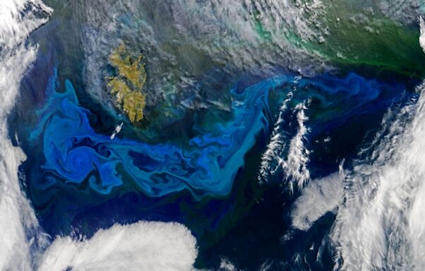
Fig. 2 The Great Calcite Belt photographed from space by the Moderate Resolution Imaging Spectroradiometer (MODIS) aboard the Aqua satellite (Stevens, 2018).
In addition to being critical for Earth’s calcite production, the unicellular organisms are also integral parts of the marine carbon cycle, providing food for predators in more nutrient-deprived environments. Coccolithophores are surrounded by scale-like structures, forming a type of armour. These structures are calcite plates, called coccoliths, and the armour is called the coccosphere (Fig. 3). Being the identifying characteristics of these organisms, these plates are directly responsible for the immense calcite contribution.

Figure 3 Images of various coccolithophore species. (a) A. specillata; (b) G. oceanica; (c) M. concave; (d) W. barnesae; (e) E. huxleyi (Sturm, 2016).
In this paper, we will be evaluating and analyzing these amazing and irreplaceable unicellular algae through the lens of mathematics. More specifically, we will be exploring the geometric intricacies of coccolithophore morphology, notably coccoliths and the coccosphere in various species of coccolithophores, as well as using well-established notions of curvature to analyze and learn about the nature of the vestigial haptonema. Furthermore, we will also be studying the growth rate of coccolithophores and the factors that affect it.
Coccolithophore Morphology
These biomineralized scales known as coccoliths are extremely diverse amongst the species that belong to the coccolithophore classification and present differently on the cell’s surface. The following section will be broken down, to discuss the geometry of individual coccoliths and then an analysis of their arrangement.
Coccolith Geometry
The shape of individual coccoliths has extraordinary differences from one species to the next, leading to numerous intricate and beautiful patterns. These structures can be more loosely classified based on their general shape and appearance. A few examples are calyptrolith, defining a basket-shaped holococcolith, open proximally (Fig. 4-A), caneolith – a disc, or bowl shape with a lath-filled central area (Fig.4-B), ceratolith delineating a horseshow or wishbone shape (Fig. 4-C), or cyrtolith, disc-shaped convex outwards often with a projecting central process (Fig.4-D) (Winter & Siesser, 2006). Do note that these are only four of the many possible coccolith assemblies.

Fig. 4 Homozygosphaera triarcha representing calyptrolith shape (A). Caneolith shape represented by Syracosphaera pulchra in B, Ceratolithus cristatus showing the horseshoe shape of ceratolith designation (C). Cyrtolith shape represented by Discosphaera tubifera in D (modified from (Dr. Jeremy R. Young)).
Although highly complex and amazingly diverse, coccoliths can be broken down into two categories; heterococcoliths and holococcoliths. The term heterococcolith is designated to coccoliths exhibiting crystal elements that differ in both size and shape, whereas holococcoliths are constructed of simply shaped tessellating crystals (Young et al., 1992). Interestingly, holococcoliths are much less common in nature even though their synthesis mechanisms may be considered simpler. This may be because their elements are often considerably smaller than the elements forming heterococcoliths, most likely causing them to disintegrate more rapidly (Winter & Siesser, 2006).
Though heterococcoliths are able to present in numerous morphologies, the simplest is described as a single disk with a ‘wall’ of rhombohedral crystals around the circumference (Fig. 5) (Winter & Siesser, 2006).

Fig. 5 Wall structure of heterococcolith of Coronosphaera mediterranea where scale bar represents 1mm (Winter & Siesser, 2006).
We can also see more complex arrangements of coccoliths, without a peripheral wall. The most common case is placoliths which are constructed by the central joining of two circular or elliptical ‘shields’ by either a solid pillar or hollow tube, as seen in in Fig. 6 (Young et al., 1992). These shields are described as proximal – the inner concave side of the coccolith, or distal – the outer convex side of the coccolith. The individual crystal elements radiate outwards from the central area which is distinctively open or closed (Fig. 7). Often composed of a singular crystal tapered near the center, but more broad towards the circumference, giving them a petal-shape, as seen in Fig. 6 and Fig. 7 coccoliths tend to radial symmetry (Winter & Siesser, 2006). This is a product of their nucleation and crystallization processes that occur along the circumference of an organic base plate. An example of an individual calcite component is seen in Fig. 8, which contains both a proximal and distal shield, and a grill flooring the central area. Although this structure is incredibly complex, with four definitive parts, it is presumed to be a single calcite crystal (Young et al., 1989).
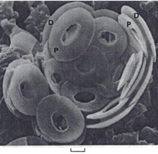
Fig. 6 Interior view of broken down coccosphere of Gephyrocaps sp. distal (D), and proximal (P) of coccoliths are joined by a short central column. Scale represents 2mm (Winter & Siesser, 2006).

Fig. 7 Representative of radial fanning pattern by individual calcite crystals in coccolith formation (BURNBTT et al.).

Fig. 8 Schematic of individual calcite crystal that radially spans to form coccoliths in reticulofenestrids, the presence of the grill determines wheter the central area is open or closed (Young et al., 1989).
Similar to heterococcoliths, holococcoliths are often composed of hexagonal prisms, rhombohedral crystals, or both. Typical arrangement is seen as the tight packing of parallel prisms, and the modification by regular absence of prisms from the pack, creating a sieve-like structure, as seen in Fig. 9. Holococcoliths can also be seen as neatly stacked rhombohedral crystals in an offset ‘checkerboard pattern’ with gaps between (Fig. 10). (Winter & Siesser, 2006)
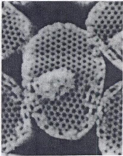
Fig. 9 Sieve-like arrangement of crystal elements in holococcolith of Sphaerocalyptra gracillima (Winter & Siesser, 2006).

Fig. 10 Euhedral crystals with rhombohedral stacking in Coccolithus pelagicus coccoliths (Winter & Siesser, 2006).
These ultrastructures of the calcite crystals that make up coccoliths are genus-specific, and are determined by nucleation and crystallization on the organic base plate (OBP), as discussed in An Analysis of the Chemistry Behind Coccolithophores (Young et al., 1992). However, the analysis of many coccoliths revealed major variations in size, mass, and segment number, even within a single coccosphere. Although, Beuvier et al. have found a correlation between coccolith mass (m), and perimeter (p), which scales linearly with the number of individual crystal components (n) in the family noelaerhabdacean, which includes the blooming Emiliania huxleyi (2019). In fact, the study suggests that the parameters are decided by the shape of the OBP in the coccolith vesicle. These relations are seen below.
m ~ p^{3.125} Where n ~ p; (Beuvier et al., 2019)
The relation between n and p implies that the width of each crystal segment remains relatively constant between any coccolithophore species, between 110 and 120 nm. Thus, it was proposed that the perimeter of the OBP fixes the number of calcite nucleation sites (one every 110-120nm) and thus pre-determines the number of crystal segments in a single coccolith. The high variation in mass and segment number within even just one coccosphere may be dependent on OBP size variability (Beuvier et al., 2019). In Fig. 11, the correlation between mass (m) and the major axis of the coccolith (a) amongst various species can be distinguished.
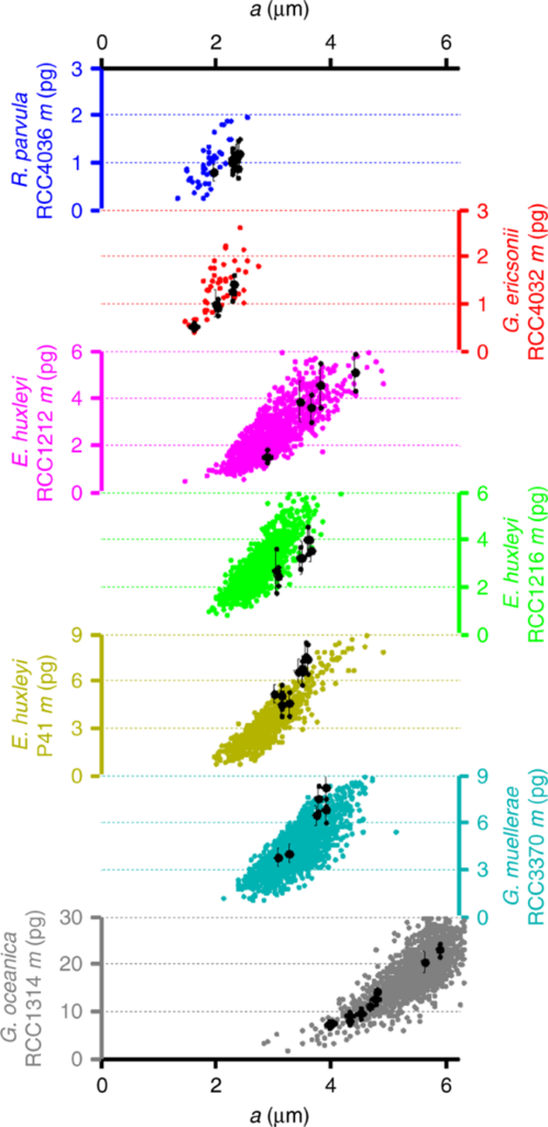
Fig. 11 Mass of coccoliths m as a function of the coccolith major axis a from polarized light microscopy (colored dots) and 3D-Xray coherent diffraction imaging (black dots) measurements (Beuvier et al., 2019).
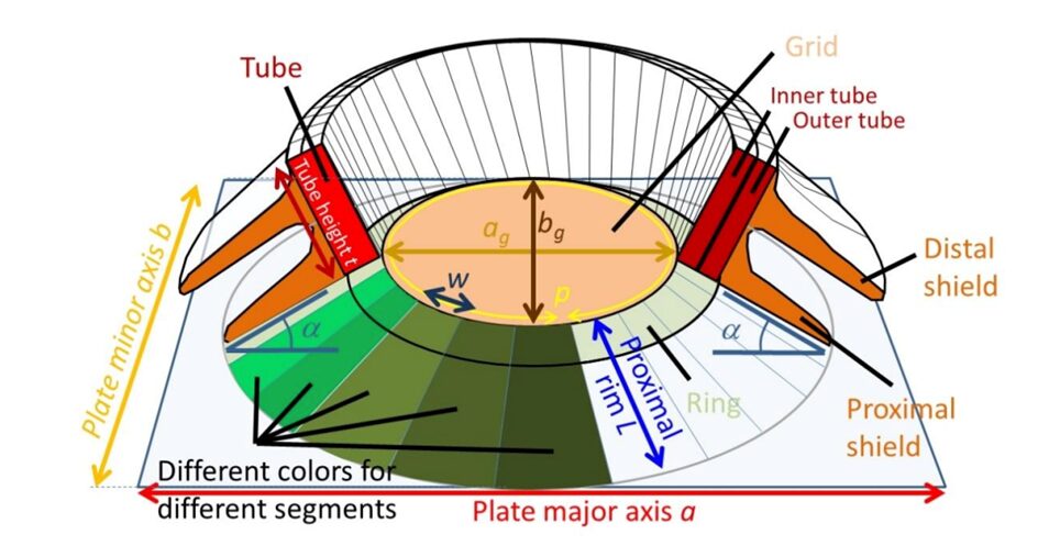
Assuming that the perimeter of the OBS is similar to that of the ‘central area’ previously discussed, and taking the shape of an ellipse, it can be calculated as below, where ag and bg represent the major and minor axis, respectively (Beuvier et al., 2019). Fig. 12 can be used as a reference to gain an understanding of the parameters mentioned.
p= π√((a_g^2+b_g^2)/2-(a_g-b_g )^2/8)
(Beuvier et al., 2019)

Fig. 12 Sketch of coccolith, displaying the parameters of study (Beuvier et al., 2019).
With this, Beuvier et al. were able to determine the positive correlation found below.
m= k_p × p^β
With mass, m, in pg, and peripheral perimeter, p, in µm.
k_p=4.92 ×10^{-2}±2.17×10^{-2}β=3.175±0.251
kp in this study was considered to be the coccolith mass index, which was fascinatingly the same for all species studied. As mentioned earlier, the number of calcite segments, n, can be linearly correlated to the peripheral perimeter as well; p = w × n, where w = 110-120 nm, the average tangential width of calcite segments at the periphery. Combining the two relations, we can compare mass and number of segments (with 95% confidence bounds) as shown below, assuming w = 112 nm, and β = 3.175.
m= k_n×n^β
k_n=4.73 ×10^{-5}±0.28×10^{-5}(Beuvier et al., 2019)
Results of this study are summarized in Fig. 13, including correlations with proximal rim length, and tube thickness. This would be an ingenious design solution if coccolithophores were somehow able to control the size of their OBP, thus controlling coccolith size to cover more or less cell surface, or their mass, to control their placement in the water column. However, there is no data supporting this theory.
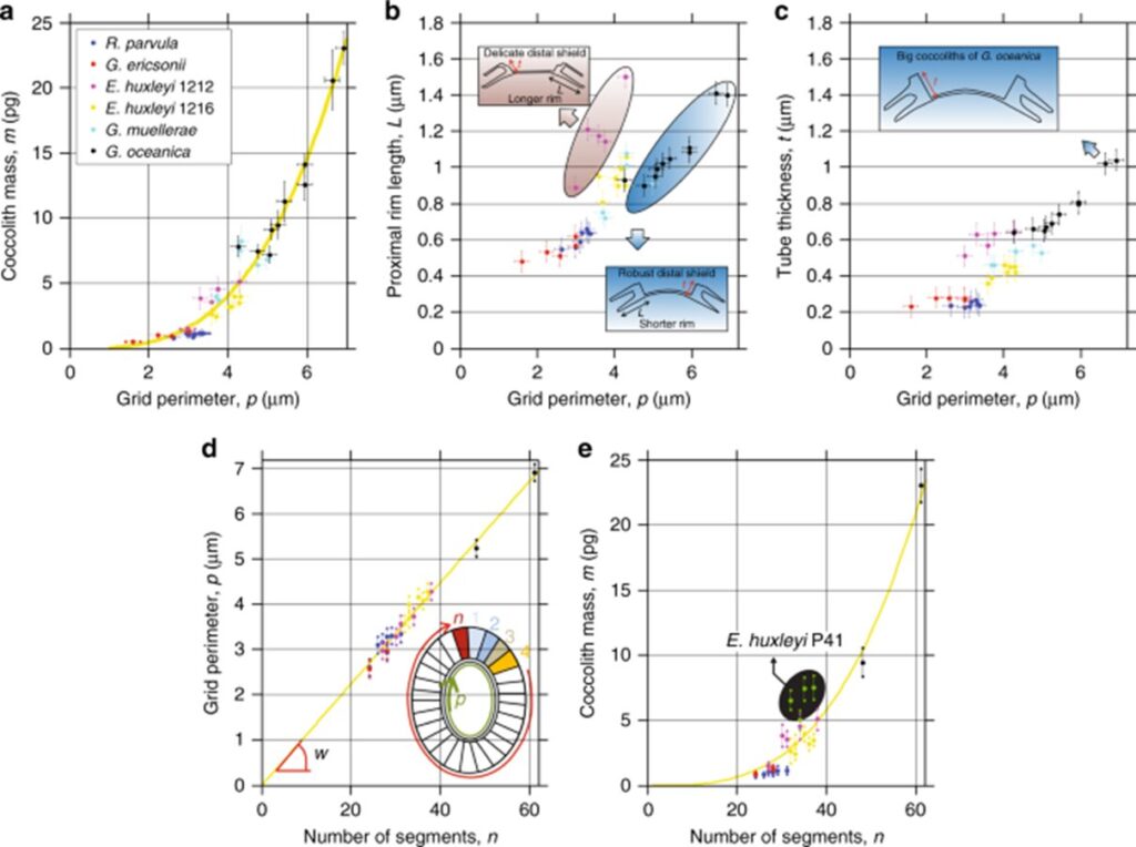
Fig. 13 Dependence of OBS on number of segments and mass of coccoliths. (a) mass of coccoliths m as function of peripheral grid perimeter p, with yellow dotted line follows m = (4.73 × 10⁻⁵) × n3.175 in pg, R2 = 95%. (b) proximal rim length L as a function of p. For given p, coccoliths with short rims showed robust distal shields, while coccoliths with long rims displayed delicate distal shields. (c) Tube thickness t as a function of p. (d) p as a function of number of segments n for coccoliths from five different coccolithophore species, equation of dotted line is p = 0.112 µm, the average width of the tube at the periphery (Beuvier et al., 2019).
Coccolith Arrangement on the Coccosphere
Although it is still a hypothesis that coccolithophores can control the size of their organic baseplate to subsequently control the size of their coccoliths, from an evolutionary standpoint, such an ability would be essential for the survival of coccolithophores. In fact, as seen in the physics and chemistry papers, these interlocked coccoliths form an armour called the coccosphere. The latter protects the cell body from mechanical and photic stresses. Coccoliths composed of calcium carbonate (CaCO3) are produced inside the cell through a process called coccolithogenesis and extruded afterward to be fixed around the protoplast. While the size of the coccoliths and their arrangement in the coccosphere might seem random, the whole process actually follows a logically designed pattern to ensure full coverage of the cell surface (Xu, Hutchins, & Gao, 2018). In fact, a study conducted by Xu et al. (2018) has found that the layout, the size, and the number of coccoliths in a coccosphere all conform with the mathematical principles and constraints behind Euler’s polyhedral formula. Based on laws derived from the formula, coccospheres were simulated by varying different parameters such as coccolith width, length, and number, and the results were compared to E. huxleyi specimens, proving that the natural evolution of coccolithophores correlates with Eulerian mathematics (Xu, Hutchins, & Gao, 2018).
To begin, it is important to observe the morphology of the coccoliths and to define the main components that will be taken into account in subsequent measurements and calculations. As shown in Fig. 14, a coccolith is ellipsoid-shaped and includes a central area surrounded by an outer distal shield (outer distal shield width written as OSW); the longest axis of the coccolith is referred to as the distal shield length (DSL), while the shortest axis is the width (DSW) (Xu et al., 2018). When coccoliths interlock with each other, they only overlap at the distal shield area and can never transect through the central area, as observed in Fig. 15 (Xu et al., 2018).

Fig. 14. Diagrams of the frontal (A) and side view (B) of a E. huxleyi coccolith, with different component labeled: the central area, the outer distal shield width (OSW), the distal shield width (DSW), the distal shield length (DSL), and the proximal shield (Xu et al., 2018).

Fig. 15 Scanning electron microscope pictures of E. huxleyi. The white bars correspond to 1 mm (Xu et al., 2018).
To model coccolith arrangements on a two-dimensional plane, polygons with various numbers of sides are used. The overlap of two neighbouring coccoliths at their distal shield forms one edge of the polygon, and three overlapped coccoliths (three overlaps of edges) intercross at a junction, forming one vertex (Fig. 16) (Xu et al., 2018). The edges form an inscribed polygon, meaning that it is placed inside the central coccolith and each vertex is on the circumference of the bigger ellipse that outlines the coccolith (Xu et al., 2018). Subsequently, coccospheres can be modeled three-dimensionally as convex polyhedra, with each face of the polyhedron corresponding to a coccolith (Fig. 17) (Xu et al., 2018). These structures follow Euler’s polyhedral formula F + V – E = 2, which describes a polyhedron with F faces, V vertices, and E edges (Xu et al., 2018). By combining the physical constraints of interlocking coccoliths and the mathematical principles of Euler’s polyhedral formula, it is possible to understand the mathematical solution behind the design of the coccosphere.
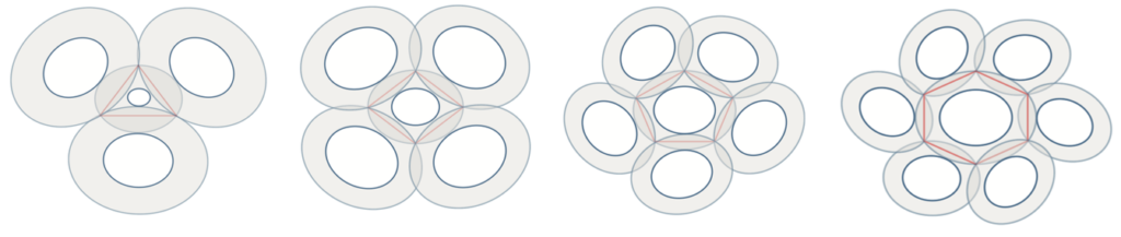
Fig. 16 Simulation of interlocked coccoliths on a 2D plane, featuring central coccoliths interlocked with three, four, five, and six others. The inscribed polygons are represented in red (Xu et al., 2018).
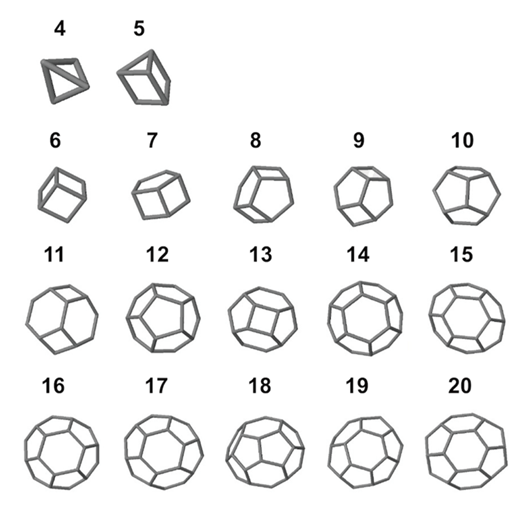
Fig. 17 Simulation of coccosphere structures represented by 3D polyhydra with 4-20 faces (Xu et al., 2018).
Xu et al. took measurements of normal coccoliths and coccospheres and established relationships between the sizes to explain the arrangement of the coccoliths. To begin, for coccoliths to be well-attached to the cell surface, they need to be interlocked closely to each other, which implies that the areas of overlap need to be maximized (Paasche, 2001). This can be achieved if the ratio between the size of the central coccolith (DSLcc) and the size of the bordering coccoliths (DSLBCs) is around 0.75-0.8; a large DSLBCs/ DSLcc results in overlaps that intersect with the central area, while a small DSLBCs/ DSLcc leads to loose interlocks (Fig. 18) (Xu et al., 2018). A tendency can therefore be observed: small central coccoliths tend to interlock with fewer and larger coccoliths, and large central coccoliths tend to interlock with more and smaller coccoliths (Fig. 16) (Xu et al., 2018). Moreover, the ratio of OSW/DSL needs to be at around 0.18 in order to sustain maximum coverage by the coccoliths, since a coccolith with an OSW that is too large can only be partly overlapped, while a small OSW does not provide enough surface for overlap (Xu et al., 2018). This ratio also takes into account the fact that shield areas need more CaCO3 to be synthesized compared to central areas, thus this ratio ensures that coccolith production can be achieved with minimum CaCO3 while maximizing coverage area (Xu et al., 2018). Furthermore, recall that coccolithogenesis is an intracellular process, so the size of a coccolith cannot exceed the diameter of the protoplast. By taking all these factors into consideration and by ensuring that Euler’s polyhedron formula is respected, Xu et al. determined that the greatest possible number of edges per coccolith is six and that at least six coccoliths are needed to construct a coccosphere.
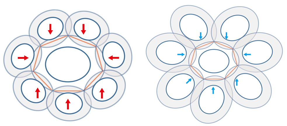
Fig. 18 Simulation of central coccoliths interlocked with seven others. The red arrows indicate overlaps that transect central areas and blue arrows indicate loose interlocks (Xu et al., 2018).
These results can be used to explain how E. huxleyi coccospheres adapt to changes in cell surface area; for instance, the full coverage of the protoplast is maintained even during cell division (Klaveness, 1972). According to Xu et al., since the minimum number of coccoliths per coccosphere is six, then E. huxleyi cell division can only be triggered when mother cells have at least twelve coccoliths such that the daughter cells can receive six coccoliths each. While the mechanism behind how the cells can precisely control this process has not yet been elucidated, it is clear that coccolithophores have found a way to increase their chances of survival by not only ensuring that they are always protected by their coccosphere but also by optimizing the effectiveness of the interlocking of the coccoliths while requiring a minimal quantity of CaCO3. Although not mathematicians, coccolithophores were millions of years ahead of us in solving the mathematical conundrum behind the design of their remarkable coccospheres!
Vestigial Haptonema
From their origin in the late Triassic period (de Vargas et al., 2007) up until one of the biggest mass extinction events known to man 66 million years ago, coccolithophores were immobile autotrophic organisms, floating around in the ocean and relying on sunlight for their photosynthetic processes. When the asteroid that wiped out the dinosaur hit our planet, huge plumes of smoke covered the sun, and thus, photosynthetic organisms struggled to survive. This put evolutionary pressures on coccolithophores, and nature had to make a decision; let coccolithophores die out along with the dinosaurs or have them adapt and hunt for their food. It was then Earth’s great calcite producers developed two flagella and a vestigial haptonema and became mixotrophs (Gibbs et al., 2020). The flagella were developed for motility whereas the haptonema, a filamentous appendage comprised of six to seven microtubules (Eikrem et al., 2017), was developed to capture prey, avoid obstacles, and adhere to substrates (Fig. 19). (For more information regarding the functions of the haptonema, refer to An Analysis of the Chemistry Behind Coccolithophores and The Physical Properties and Interactions of Coccolithophores.
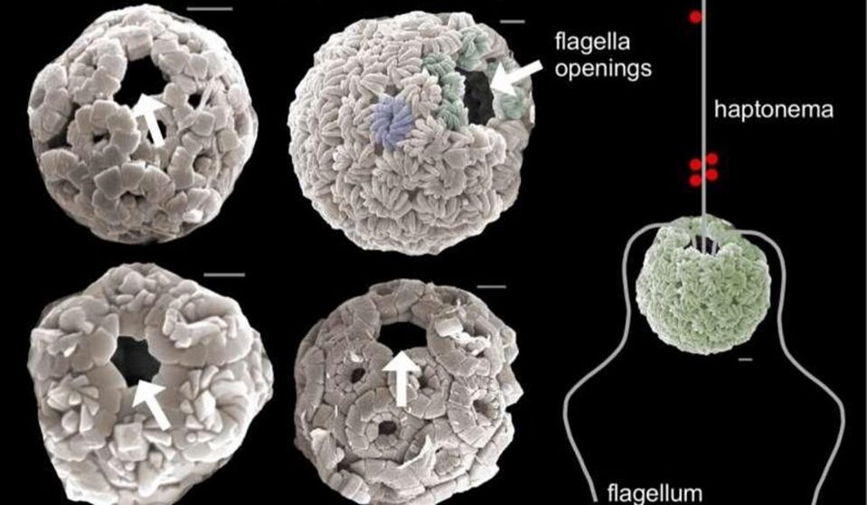
Figure 19 Scanning electron microscope images of the flagella opening in coccolithophores and the flagella and vestigial haptonema arrangement in these organisms (Riverside, U. of C., 2020).
The haptonema is characterized by its ability to both coil and bend depending on what the cell needs. In the case of obstacle avoidance, the organelle will coil tightly and incredibly quickly (1/60 – 1/100 s) (Tsuji & Yoshida, 2017), whereas in the case of prey capture, it will bend gradually to deliver the food aggregate collected to the side of the cell where the captured food is then ingested by the organism (Fig. 20). One common denominator in both processes is the curving of the haptonema. This implies that there is a radius of curvature that we can calculate (Fig. 22), which allows us to quantitatively measure the behaviour of this organism and more specifically, this organelle, in different conditions and environments.

Figure 20 Sketch of vestigial haptonema prey capture process. (c)Food particles (prey) are captured on the haptonema, which then move proximally to the particle aggregating center. (d) The food agregate then moves distally to the tip of the haptonema. (e) The haptonema first begins to bend proximally, but eventually bends completely to wrap around cell and deliver food aggregate to the cell to be ingested via phagocytosis. (f) Large particle engulfment (Dölger et al., 2017).
As previously mentioned, the haptonema curvature is measured using the radius of curvature (Fig. 22). This was done by inscribing circles along the curved portions of the haptonema and assigning a function y = f(x) to these circles. The radius of curvature is also known as the reciprocal of the curvature, a measure of the average change of the curve’s direction per unit of arc length (Vert, 2023), is given by the following equation:
ρ=(1+(y')^2 )^{3/2}/|y"| Eq. 1 (Adapted from Vert, 2023)
As a result, the curvature is given by the equation:
κ=y"/(1+(y')^2 )^{3/2}Eq. 2 (Adapted from Vert, 2023)
The above equations are the final product of the derivations made. To understand where they come from, we must first observe the components of Figure 21:

Figure 21 Curvature and radius of curvature components of a non-circular curve over the arc length . Let c1 and c2 be the centers of the circles generated at points P1 and P2, respectively, with radii r1 and r2, respectively. Let a represent the angle formed by the intersection of the tangent of each circle with the horizontal axis, and Da represent the difference of said angles (Vert, 2023).
Consider the yellow curve above and let us model it after a curved portion of a coccolithophore’s haptonema. We know, from basic geometry, that the arc length is given by the following equation:
∆s=ρ∙∆α
Eq. 3.1 (Vert, 2023)
Where ρ is the radius of curvature.
This equation can be rearranged to yield the equation of the curvature (κ) of a circle:
κ=1/ρ=∆α/∆s
Eq. 3.2 (Vert, 2023)
From equation 3.2, we see that there is a ratio between the change in angle, Da, and the arc length, Ds. In non-circular arc lengths, such as the one in Figure 21, we see that as P2 approaches P1 along the curve, the aforementioned ratio approaches a limit (Vert, 2023). This limit is called the limit of curvature at a particular point, given by the following equation:
κ=lim_{∆s→0} ∆α/∆s=dα/dsEq. 4 (Vert, 2023)
We know that the slope of the tangent line, m, is given by the tangent of the angle of inclination, so,
m=tan(α)
Eq. 5 (Vert, 2023)
Then, from calculus, we have that:
m=dy/dx
tan(α)=y'
α=arctan{(y')}Eq. 6 (Vert, 2023)
By differentiating both sides with respect to x, we get:
dα=y"/(1+{(y')}^2 ) dxEq. 7 (Vert, 2023)
We also know that in the xy-plane, the differential arc length, ds, is given by:
ds=√(1+{(y')}^2 ) dxEq. 8 (Vert, 2023)
Since we have concluded that the curvature is given by the ratio of the angle difference and the differential arc length using Equation 4, we have that the curvature is given by Equation 2, its reciprocal, and the radius of curvature is given by Equation 1.
Now that the proper equations have been derived, we can evaluate the curvature of the haptonema at any point along the organelle. In the case of Fig. 22, this is done at the dark blue and red points. From this newly acquired information, one can construct a graph plotting the curvature of the haptonema against the distance of the curvature from the base of the organelle, a value known as the bend propagation (Fig. 23) (Nomura et al., 2019).
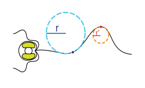
Figure 22 Radius of curvature of the curved regions of the vestigial haptonema (Nomura et al., 2019).
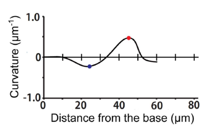
Figure 23 Bend propagation of haptonema (Nomura et al., 2019).
Calculating the curvature, as well as the radius of curvature of the haptonema allows scientists to quantitatively measure how this organelle behaves in the presence of different stimuli, in different conditions, and more, which helps with the understanding of the behaviour of this filamentous appendage. New trends may emerge which can help scientists gain valuable insight on this structure. For example, in a study conducted by Nomura et al. in 2019, the coiling mechanism of the haptonema was investigated using drugs that would affect the microtubules in haptonema coiling. Three drugs were used to do so: DMSO, Taxol, and Nocodazole (Nomura et al., 2019). The curvatures of the haptonema in the presence of these drugs were calculated and the associated bend propagations were plotted (Fig. 24).
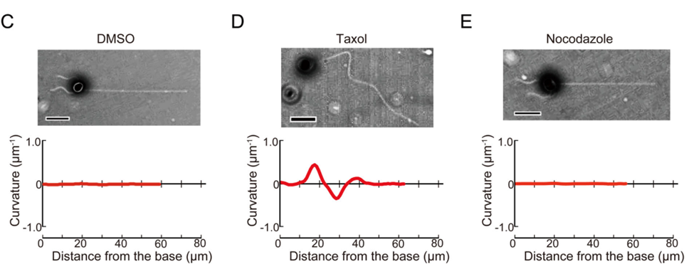

Figure 24 Bend propagation of the vestigial haptonema in the presence of various microtubule-affecting drugs (Nomura et al., 2019).
With the help of these results, the Ca2+-dependent coiling mechanism of the haptonema was deduced which led to numerous breakthroughs in our understanding of this filamentous appendage. (For more information regarding the breakthroughs of the mechanism of haptonema coiling, refer to The Physical Properties and Interactions of Coccolithophores. Essentially, with the help of the curvature and our ability to calculate it, one of nature’s most ingenious design solutions is beginning to become understood.
These results highlight how a seemingly unimportant measurement, whose derivation is simple, can lead to scientific breakthroughs in the understanding of the organelle that allowed the world’s greatest calcite producers to survive the Cretaceous-Paleogene extinction event 66 million years ago. This also allows for quantitative measurement of this organelle’s behaviour, which can be used to identify new trends and, in turn, learn more about this wonderful unicellular organism that is the coccolithophore.
Growth Rate of Coccolithophores
Dependence on cell diameter
There are many coccolithophore species with different surface morphology and cell size, which vary from 2-42 micrometers in cell diameter. However, according to the analysis done by Villiot et al, the majority of coccolithophore species (~71%) are smaller than 10 μm in diameter, whereas approximately half of the species (~52%) have cell dimensions between 5 and 10 μm (Fig. 25A). The size ratio between the diploid and haploid life stages also shows no significant difference, with both stages having similar median cell sizes around 7–8 micrometers. This suggests that the coccolithophore is constrained in its size, along with most nanoplankton. Especially, the ubiquitous species which often show dominance in the present-day ocean like E. huxleyi or G. oceanica have generally smaller and more restricted cell sizes compared to other coccolithophores. Further analysis regarding the surface area-to-volume (SA:V) ratio shows that the majority of the coccolithophore (~72%) have an SA:V ratio above 0.6 μm-1 (Fig. 25B). This restricted cell size seen in the coccolithophore is a design solution that makes coccolithophores good competitor for resource acquisition in low nutrient and low-light environments. By having small cells and high cell SA:V ratios, the coccolithophore is adapted for passive nutrient diffusion and for limiting the package effect for light harvesting. In fact, coccolithophore consistently shows the highest species diversity in oligotrophic environments, such as the central subtropical gyres (Villiot et al, 2021).
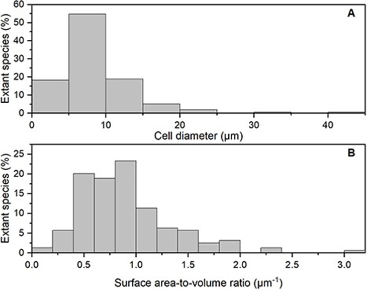
Fig. 25 Frequency histogram of the percentage of extant species in different bins of (A) cell size (μm) and (B) surface area to volume ratio (μm-1) (Villiot et al, 2021).
Interestingly, the coccolithophore size-scaling of growth rate also matches with the basic metabolic theory. The relationship between growth rate and cell volume (Fig. 26) shows an allometric relationship of exponent -0.19. This relationship seen in coccolithophore is very close to metabolic theory, which has an exponent of -0.25, while it is -0.13 for diatoms grown at optimal growth temperatures and -0.15 for all types of algae (Villiot et al, 2021). Differences in growth rate scaling patterns among these phytoplankton groups help us understand the competition between groups and the dominance of certain groups in a specific environment (Dutkiewicz et al., qtd in Villiot et al, 2021). Although smaller cells have higher growth rate, recent studies have revealed that bloom-forming phytoplankton species are composed of intermediate cell sizes, with bloom-forming coccolithophore species such as Gephyrocapsa oceanica (∼300 μm3), Emiliana huxleyi (∼50 μm3) and Syracosphaera bannockii (∼400 μm3) (Villiot et al, 2021). This might be due to the grazer control effect, for example, by zooplankton. In their natural environment, as smaller species become more abundant, the grazer of these species also increases, consequently decreasing their net growth rate. This allows for the coexistence of different phytoplankton species in the same environment (Dutkiewicz et al., 2020).

Fig. 26 Relationship between growth rates (d−1) and cell volumes (μm3) for the nine coccolithophore strains (Villiot et al, 2021).
Dependence on temperature
The relationship between growth rate and temperature is studied in five different species of coccolithophore measured at different temperatures between 6 °C and 25 °C. The observed optimal growth temperature (Fig. 27A) correlates with the biogeography of these coccolithophores. The species C. braarudii grew relatively best at low temperatures, its growth rate decreased much more slowly than the growth rate of Emiliania huxleyi, while the other species did not grow at all at 6°C. This is consistent with C. braarudii abundance in sediment trap samples from the northern North Atlantic. The two strains of C. leptoporus showed somewhat different temperature optima at 12°C and 20°C, however, they did not grow at 6°C or 25 °C and barely grew at 9°C. The species C. leptoporus is a cosmopolitan species and it can grow in a rather large temperature range. In addition, G. oceanica and S. pulchra have the highest growth rate at 25°C, while they did not grow at all at temperatures lower than 9°C. Again, this is consistent with the biogeographical distribution toward the Earth’s equator of G. oceanica and the subtropical abundance of S. pulchra. Overall, we see the partition of niches seen in coccolithophore, since each species is optimized to grow at a specific temperature and did not grow in others, which allows them to minimize interspecific competition. The only exception is the species E. huxleyi where it was seen to grow at all studied temperatures. Since E. huxleyi is the most abundant species of coccolithophore in the modern ocean, this growth trend can somewhat explain its worldwide domination. In general, the growth rate decreases as the temperature decreases, fitted quite similarly in both linear and exponential functions of temperature (Fig. 27B) (Buitenhuis et al, 2008).
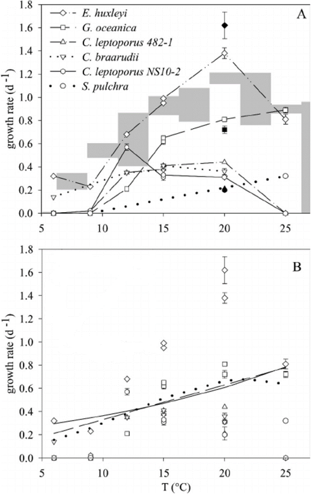
Fig. 27 Growth rates of coccolithophores as a function of temperature, (A) different species of coccolithophore, (B) fitted function that show growth rate trend (Buitenhuis et al, 2008).
Dependence on CO2 concentration
In coccolithophores, the growth rate increases with increased CO2 concentration before 70 nmol l−1 H+ and then drops significantly after this point. It is suggested that at low CO2 concentration, the CO2 substrate is the main driver for growth rate and not pH, thus growth rate goes up since this substrate is beneficial for processes like photosynthesis. While at high CO2, pH is the main driver for growth rate and therefore causes the drop observed after 70 nmol l−1 H+ in the case of coccolithophores (Fig. 28A). This optimum curve pattern is also observed in other phytoplankton taxa, like in cyanobacteria or diatoms (Fig. 28B, C). However, in other phytoplankton, the optimal growth rate is reached at a higher H+ concentration compared to coccolithophore, like 170 nmol l−1 H+ for three species of diatoms. This trend is shown more clearly when putting all three taxa together on the same conceptual graph (Fig. 28D) (Paul and Bach, 2020). Calcifying haptophytes like the coccolithophore are known to be particularly sensitive to ocean acidification, which affects their calcium carbonate formation. As seen in our last paper about chemistry, voltage-gated proton channels, which help to regulate cell pH homeostasis and export of H+ during calcification, are highly sensitive to the proton gradient. Here, the optimum growth curves further confirm the potential negative effect that ocean acidification will have on phytoplankton in general and coccolithophores in particular.
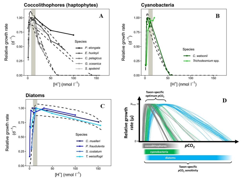
Fig. 28 Relative growth rate of different phytoplankton across a wide range of H+ concentrations ([H+]) for (A) coccolithophore, (B) cyanobacteria, (C) diatoms. And (D) Conceptual figure of what multiple pCO2 reaction norms for a variety of species/taxa could look like (Paul and Bach, 2020).
Coccolithophore’s Efficient Use of Nutrients
Although there is variability within different species of coccolithophores (Fig. 29A,B), overall, we see a similar organic carbon to nitrogen (C:N) ratio between coccolithophores and the other phytoplankton like diatoms, dinoflagellates and green algae, lower C:N ratio than red algae and higher than cyanobacteria (Fig. 30). However, coccolithophores unlike other key functional phytoplankton groups, have two pools of cellular carbon, both organic and inorganic, and their PIC:POC ratios are close to 1 (Fig. 29C), highlighting that coccolithophores fix at least an equal amount of their cellular organic carbon as CaCO3. Because of the significant cellular investment in making CaCO3, it could be expected that this requires additional metabolic or nutritional resources over and above that found in noncalcifying phytoplankton. However, the organic C:N content of coccolithophores is the same as for other phytoplankton groups, it is even more obvious by the rough doubling of C:N ratios with the inclusion of their inorganic C (Fig. 30). This implies their efficient utilization of N compared to other phytoplankton; it has been shown that E. huxleyi blooms can occur in environments under conditions of N limitation. This is a design solution by coccolithophores that allows them to effectively compete for and utilize organic nutrient sources (Villiot et al, 2021).
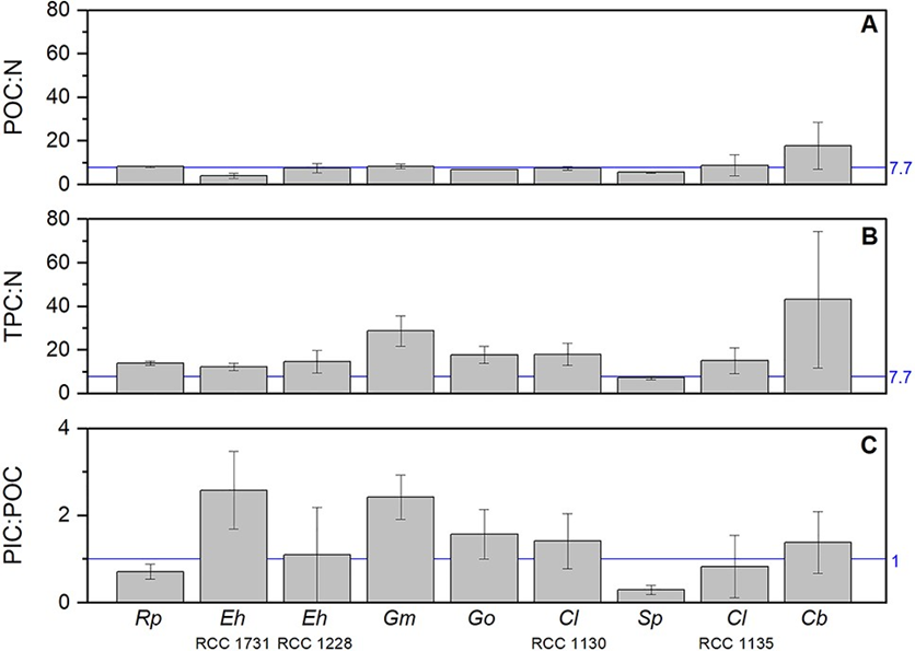
Fig. 29 Elemental stoichiometric ratios (mol mol−1) for the nine coccolithophore strains. Ratios are given for: (A) particulate organic carbon (POC) to nitrogen (N); (B) total particulate carbon (TPC) to nitrogen (N); (C) particulate inorganic carbon (PIC) to particulate organic carbon (POC) (Villiot et al, 2021).

Fig. 30 Comparative analysis of carbon to nitrogen (C:N) ratios (mol mol−1) for different phytoplankton groups (Villiot et al, 2021).
Conclusion
Faced with the harsh environmental conditions of the vast ocean, coccolithophores have evolved to find the most optimal mechanisms to protect themselves and to perform activities that are essential for their survival, allowing them to thrive and become the biggest calcite producers of the marine ecosystem.
Their biological armour, the coccosphere, is composed of coccoliths that come in various shapes and sizes and are formed through a genus-specific calcite crystallization process. The mass and the perimeter of the coccoliths are shown to depend on the size of the organic base plate, where calcite nucleation is initiated. Although still a hypothesis, this dependence could allow the organism to control the size of its coccoliths or their mass, which subsequently gives them the ability to control their vertical displacement. From the perspective of Eulerian mathematics, the coccolithophores must have such an ability to control the synthesis of their coccoliths as well as their arrangement in the coccosphere, since simulations of coccospheres based on Euler’s polyhedral formula have shown that the size, the number, and the layout of coccoliths in coccolithophore samples were engineered to ensure the full coverage of the protoplast. The well-designed coccosphere can adapt to changes in cell surface area and allows coccolithophores to minimize CaCO3 consumption.
Moreover, our understanding of the mathematical principles behind the arrangement of coccoliths could be useful for the modeling of extinct coccolithophore species, since coccolithophore fossils are always found as detached coccoliths and not as intact coccospheres (Sheward, 2016).
When it comes to prey capture and locomotion, coccolithophores found yet again an ingenious solution: the vestigial haptonema. It has the ability to coil and bend repetitively without breaking, allowing the coccolithophore to avoid obstacles and capture prey. These movements can be analyzed through mathematical formulas to better understand the mechanism behind the haptonema.
Finally, the growth rate of coccolithophores is regulated by several factors such as geometric constraints, basic metabolic theory, water temperature, and CO2 concentration. The fact that their growth rate is adapted to these varying conditions allows coccolithophores to acquire nutrients and make use of their resources effectively to ensure their survival and to bloom.
By studying coccolithophores through the lenses of physics, chemistry, and mathematics, it has become clear that it is no coincidence that these creatures have become such an integral part of the marine ecosystem; they have found astonishing design solutions to overcome the obstacles that were presented to them.
References
Beuvier, T., Probert, I., Beaufort, L., Suchéras-Marx, B., Chushkin, Y., Zontone, F., & Gibaud, A. (2019). X-ray nanotomography of coccolithophores reveals that coccolith mass and segment number correlate with grid size. Nature communications, 10(1), 751.
Buitenhuis, E. T., Pangerc, T., Franklin, D. J., Le Quéré, C., & Malin, G. (2008). Growth rates of six coccolithophorid strains as a function of temperature. Limnology and Oceanography, 53(3), 1181-1185. https://doi.org/10.4319/lo.2008.53.3.1181
de Vargas, C., Aubry, M.-P., Probert, I., & Young, J. (2007). Chapter 12 – origin and evolution of coccolithophores: From coastal hunters to oceanic farmers. In P. G. Falkowski & A. H. Knoll (Eds.), Evolution of Primary Producers in the Sea (pp. 251–285). Academic Press. https://doi.org/10.1016/B978-012370518-1/50013-8
Dölger, J., Nielsen, L. T., Kiørboe, T., & Andersen, A. (2017). Swimming and feeding of mixotrophic biflagellates. Scientific Reports, 7(1), 39892. https://doi.org/10.1038/srep39892
Dutkiewicz, S., Cermeno, P., Jahn, O., Follows, M. J., Hickman, A. E., Taniguchi, D. A. A., & Ward, B. A. (2020). Dimensions of marine phytoplankton diversity. Biogeosciences, 17(3), 609-634. https://doi.org/10.5194/bg-17-609-2020
Eikrem, W., Medlin, L. K., Henderiks, J., Rokitta, S., Rost, B., Probert, I., Throndsen, J., & Edvardsen, B. (2017). Haptophyta. In J. M. Archibald, A. G. B. Simpson, & C. H. Slamovits (Eds.), Handbook of the Protists (pp. 893–953). Springer International Publishing. https://doi.org/10.1007/978-3-319-28149-0_38
Gibbs, S. J., Bown, P. R., Ward, B. A., Alvarez, S. A., Kim, H., Archontikis, O. A., Sauterey, B., Poulton, A. J., Wilson, J., & Ridgwell, A. (2020). Algal plankton turn to hunting to survive and recover from end-Cretaceous impact darkness. Science Advances, 6(44), eabc9123. https://doi.org/10.1126/sciadv.abc9123
Klaveness, D. (1972). Coccolithus huxleyi (Lohm.) Kamptn. II. The flagellate cell, aberrant cell types, vegetative propagation and life cycles. British Phycological Journal, 7, 309-318. https://doi.org/10.1080/00071617200650321
Nomura, M., Atsuji, K., Hirose, K., Shiba, K., Yanase, R., Nakayama, T., Ishida, K., & Inaba, K. (2019). Microtubule stabilizer reveals requirement of Ca2+-dependent conformational changes of microtubules for rapid coiling of haptonema in haptophyte algae. Biology Open, bio.036590. https://doi.org/10.1242/bio.036590
Paasche, E. (2001). A review of the coccolithophorid Emiliania huxleyi (Prymnesiophyceae), with particular reference to growth, coccolith formation, and calcification-photosynthesis interactions. Phycologia, 40(6), 503-529. https://doi.org/10.2216/i0031-8884-40-6-503.1
Paul, A. J., & Bach, L. T. (2020). Universal response pattern of phytoplankton growth rates to increasing CO2. New Phytologist, 228(6), 1710-1716. https://doi.org/10.1111/nph.16806.
Radius of curvature formula—Learn formula for radius of curvature. (n.d.). Cuemath. Retrieved November 29, 2023, from https://www.cuemath.com/radius-of-curvature-formula/
Riverside, U. of C.-. (2020). To survive asteroid impact, algae learned to hunt. https://phys.org/news/2020-10-survive-asteroid-impact-algae.html
Sheward, R. (2016). Cell size, coccosphere geometry and growth in modern and fossil coccolithophores
Stevens, J. (2018, January 6). South Atlantic Abloom [Article]. Nasa Earth Observatory; Nasa. https://earthobservatory.nasa.gov/images/91521/south-atlantic-abloom
Sturm, R. (2016, February 5). Coccoliths: Tiny fossils with immense paleontological importance. Deposits Mag. https://depositsmag.com/2016/02/05/coccoliths-tiny-fossils-with-immense-paleontological-importance/
Tsuji, Y., & Yoshida, M. (2017). Biology of haptophytes: Complicated cellular processes driving the global carbon cycle. In Advances in Botanical Research (Vol. 84, pp. 219–261). Elsevier. https://doi.org/10.1016/bs.abr.2017.07.002
Vert, J. (2023). Curvature and radius of curvature | differential calculus review at mathalino. MATHalino – Engineering Mathematics; Drupal. https://mathalino.com/reviewer/differential-calculus/curvature-and-radius-curvature
Villiot, N., Poulton, A. J., Butcher, E. T., Daniels, L. R., & Coggins, A. (2021). Allometry of carbon and nitrogen content and growth rate in a diverse range of coccolithophores. Journal of Plankton Research, 43(4), 511-526. https://doi.org/10.1093/plankt/fbab038.
Winter, A., & Siesser, W. G. (2006). Coccolithophores. Cambridge University Press.
Xu, K., Hutchins, D., & Gao, K. (2018). Coccolith arrangement follows Eulerian mathematics in the coccolithophore Emiliania huxleyi. PeerJ, 6, e4608. https://doi.org/10.7717/peerj.4608
Young, J. R., Crux, J., & van Heck, S. (1989). Observations on heterococcolith rim structure and its relationship to developmental processes. Nannofossils and their applications. Ellis Horwood, Chichester, 1-20.
Young, J. R., Didymus, J. M., Brown, P. R., Prins, B., & Mann, S. (1992). Crystal assembly and phylogenetic evolution in heterococcoliths. Nature, 356(6369), 516-518.