Abstract
Artificial neural networks are used to mimic the functionalities of the brain via computing systems. This paper will first examine the general structure and function of artificial neural networks, as well as their similarities and differences to the brain’s neural network, after which they are modelled. Then, the essay will discuss how neural networks can be used to simulate olfaction processes by looking at the olfactory system of a fly. It was found that the system rearranged itself to form a structure similar to that of a fly brain, implying that the brain is optimally designed for the process of olfaction. Afterwards, the paper explores how artificial neural networks are used to simulate the vision process by analyzing the design of micro aerial vehicles inspired by the flight control techniques found in honeybees. Finally, the paper will look at taste reception and how an artificial neural network (ANN) was used to model neural computation of tasting in rats.
Introduction
The brain is the most complex organ of the body, controlling functions such as thought, motor skills, vision, breathing and memory. Currently, our understanding of the complete functionality of the brain is quite limited. Hence, mimicking its intricate circuitry via computer modelling has proven to be quite difficult. The use of artificial neural networks comes to fruition when attempting to overcome these challenges. Neural networks are computing systems that take inspiration from inner workings of the brains of living beings to model the structure and flow of information. Through the application of machine learning, these systems attempt to process information in a similar method to the brain. This technology can be used for various applications, including the simulation of numerous sensory functionalities in animals such as olfaction, vision, and taste.
Artificial Neural Networks – An Overview
Although computers continue to evolve and gain new abilities at rapid rates, they are far from being able to perform certain tasks at the same level as the brain of a living being. Computers are incapable of acquiring new capabilities without some kind of software update, unlike the brain, which can continuously learn and whose abilities to perceive the world are constantly modified by past experience (Krogh, 2008). The closest researchers have come to being able to model how living beings learn and respond to stimuli is through artificial neural networks.
What are Artificial Neural Networks?
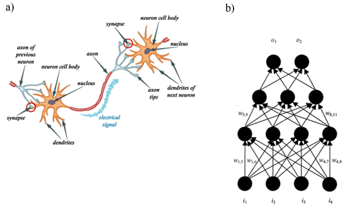
The brain consists of a highly interconnected network of neurons, which pass information between one another by sending electric pulses through their axons, synapses, and on to the dendrites of the next neurons (Figure 1a). Artificial neural networks are modeled after the brain’s natural neural network and are made to simulate the electrical activity of the brain and nervous system (Krogh, 2008). Processing elements (called neurodes or perceptrons) are interconnected to each other, mimicking a network of neurons (Figure 1b). Perceptrons in the artificial network are typically arranged in a layer, or vector, where the output of one layer serves as the input of the next, or possibly other layers, and so on. Additionally, a perceptron can be connected to some or all of the perceptrons in the next layer, simulating the complexity of synaptic connections in the brain (Walczak & Cerpa, 2003). An artificial neural network can have anywhere from dozens to millions of perceptrons (Marr, 2018). The initial input is usually some sort of sensory signal, such as an image, sound waveform, or spectrogram, and the output units are interpreted as probabilities of target classes, meaning that each input ends up being sorted into the output condition that best suits it, depending on what task the network is trained to carry out (Kell & McDermott, 2019).
How do they work?
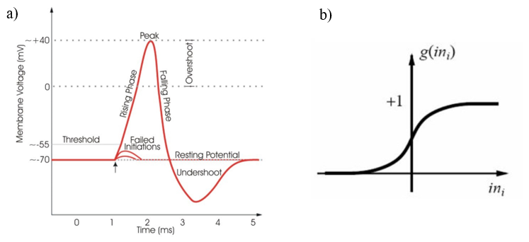
In the brain, a neuron will receive excitatory or inhibitory signals from many other neurons. If the strength of the combined signals passes a certain activation threshold, then the neurons will fire an action potential, causing the signal to be passed on to further neurons (Figure 2a) (Hollander, 2018). Artificial neural networks mimic this process by defining the connections between units with weights, meaning that some connections have more influence than others on the system. The input values to a processing element are each multiplied by their associated connection weights, and since each connection carries a different weight, this simulates the strengthening of certain neural pathways in the brain over others (Walczak & Cerpa, 2003). This is thus how learning is emulated in artificial neural networks. All of the weight-adjusted input values are then summed to produce a single overall input value to the neurode. The neurode then puts this total input value through a transfer function to produce its output, which becomes an input for the next processing layer (Walczak & Cerpa, 2003). The transfer function is usually some kind of nonlinear function, such as a sigmoid function, the differentiable approximation of a step function, which mimics the binary method that neurons use to determine whether or not they will fire an action potential (Figure 2b). If the total input value is above a certain threshold, determined by the sigmoid function, the output will trend towards one, and if not, it will trend towards zero (Krogh, 2008). The process repeats itself between each layer of processing elements until a final output value, or vector of values is produced by the network (Walczak & Cerpa, 2003).
In order for artificial neural networks to learn, they must be trained by inputting large amounts of information called a training set. For example, to teach an artificial neural network to differentiate between a cat and a dog, the training set would consist of thousands of images tagged as either cat or dog that the network can use to learn. Once a significant amount of data has been imputed, the network will try to classify future data based on what it thinks it is seeing (Marr, 2018). To do this, it uses a back-propagation learning algorithm called a gradient descent. First, all of the weights in the connections of the network are set to small random numbers. For each input example, the network gives an output that is compared to the desired output, which is usually the human-provided description of what should be observed (Krogh, 2008). The algorithm measures the difference between its output and the desired one and uses this information to go back through the layers and adjust the values of the weights, in order to get a better result. This trial process is repeated each time an example is presented, such that the error gradually becomes smaller until the total error value of the network is minimized as much as possible, meaning that the output of the network can adequately match the desired output (Marr, 2018).
How do they differ from Natural Neural Networks?
One of the most important differences between artificial neural networks and the perceptual systems of living beings lies in the inflexibility of how artificial networks are trained to learn. The artificial neural network is usually limited to performing specific tasks of which it is trained, and although things learned for one task can transfer to others, this still would require the introduction of new training examples to adapt to the new task (Kell & McDermott, 2019). This is very different from the way that brains can use one input, like an auditory or visual signal, to answer a wide range of questions or perform a wide range of tasks. Additionally, the neuroplasticity of the brain, meaning its ability to adapt its structure and function, allows for new neural connections to be made and old ones to be lost or for certain areas to move and change function based on their importance (Kell & McDermott, 2019). The process of learning builds on information that is already stored in the brain, and deepening knowledge through repetition allows for tasks to be executed automatically, as well as being able to apply that existing knowledge to new unlearned tasks. On the other hand, although the weights between connections can change through the training process, no further connections or units can be added or removed from artificial neural networks once the predefined model is established (Nagyfi, 2018). Because of this, changing the weights may yield the optimal performance for that specific network model, but this only represents one of the infinite approximations to a solution that can come from using different models with different amounts of perceptrons and connections between them, just as there are many solutions for the same problem in real life (Nagyfi, 2018).
The applications of artificial neural networks span across many fields of research in science, medicine and engineering. They can be used to classify information, predict outcomes and cluster data (Krogh, 2008). The next part of this paper will focus on how artificial neural networks are used in sensory processing, with 3 concrete examples of how the sensory systems of certain animals have been used as models for artificial neural networks with applications in engineering.
Artificial Neural Networks Designed for Olfaction
One application of artificial networks is to mimic olfactory sensation in animals. Using machine learning, a model can teach itself to smell within just a few minutes (Michalowski, 2021). In one study, they sought to research how such olfactory systems would evolve in artificial neural networks when trained to perform olfactory tasks (P. Y. Wang et al., 2021)
Olfaction in animals
Although morphologically dissimilar, and separated by 500 million years of evolution, fruit flies and mice have analogous olfactory circuitry (P. Y. Wang et al., 2021). This similarity is due to the process of convergent evolution, where they both independently evolved these systems to perform similar tasks.
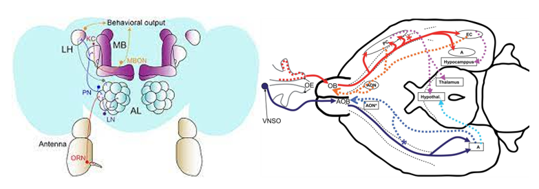
In fruit flies, olfaction is initiated by the binding of different odourants to their olfactory receptors on the surface of their antennae (P. Y. Wang et al., 2021). Olfactory receptor neurons (ORNs) will then express one of 50 different olfactory receptors (ORs). When receptor neurons express the same receptor, they converge onto a glomerulus within the antennal lobe of the brain. Then, projection neurons (PNs) send axons to neurons in the lateral horns where it mediates innate behaviours. Signals are also sent to Kenyon cells (KCs) in the mushroom body (MB) where it is translated into associative memories and learned behaviours (Figure 3).
The system is very similar to that of a mouse, where neurons expressing a given scent receptor converge on to a fixed glomeruli in the olfactory bulb (similar to the antennal lobe of an insect) (P. Y. Wang et al., 2021). The PNs then send signals to the primary olfactory cortex where they synapse onto piriform neurons (Figure 3).
Modelling Olfaction
These similarities lead us to believe that the olfactory circuits in an artificial network would also evolve to resemble the structure found in the brain. In the study, they assembled a network of artificial neurons mimicking that of the fruit fly olfactory system (Michalowski, 2021). Giving it the same number of neurons as the fruit fly system, but with no inherent structure. Scientists had asked the network to assign data representing different odours to different categories and to correctly organise single odours and mixtures of odours, something the brain is uniquely good at doing. For example, as Yang states, if you were to combine the scents of different apples, the brain would smell apples (Michalowski, 2021). In contrast, if you were to combine two photographs of cats pixel by pixel, the brain will no longer see a cat (Michalowski, 2021). This feature of the olfactory system captures the complexity that must be mimicked in these networks. Within a few minutes, the artificial network was able to organize itself, forming new connections, and what emerged was a structure very similar to that of the olfactory circuit of a fruit fly.
Such principles can also be applied to model foraging for different animals. For example, in one design, they mimicked the strategies employed by flying insects when foraging (Rapp & Nawrot, 2020). Using the spiked-based plasticity rule, the model quickly learned how to associate olfactory cues paired with food. Spiked based plasticity is the process in which the strength of connections between neurons and the brain adjust, based on the timing of a particular neurons’ output and input potentials (the spikes), which they mimicked through spiked based machine learning (Rapp & Nawrot, 2020). Without training the system, they found that it could recall memories to detect cues.
The convergence of the artificial olfactory neural networks to be similar to that of the biological olfactory circuitry in animals shows us that the brain interprets olfactory information optimally (Michalowski, 2021). Whereas evolution found its organization through the process of mutation and natural selection, the artificial network created its design via standard machine learning algorithms (P. Y. Wang et al., 2021).
Artificial Neural Networks Designed for Vision
Due to their small size and limited computation capability, it is difficult for micro aerial vehicles (MAVs) to execute precise flight maneuvers using visual information. To overcome this challenge, researchers have analyzed the visual systems in flying insects, such as honeybees, as they embody several properties desirable for MAVs, including agile flight, low weight, small size, and low energy consumption. With the data collected from the honeybee, engineers can mimic the insect’s methods of perceiving its surroundings during flight to design functional MAVs using artificial neural networks.
Angular Velocity Decoding Model (AVDM)
According to behavioural experiments on honeybees, their ability to estimate and regulate angular velocity allows them to control their flight and perform delicate maneuvers. Electrophysiological research further suggests that the electrical activities of some neurons in the honeybee’s ventral nerve cord increase as the angular velocity of the stimulus grating movement increases (H. Wang et al., 2020). Using these concepts, engineers have developed an angular velocity decoding model (AVDM) to design MAVs’ flight control system, which relies on visual signals. This complex model explored in H. Wang et al.’s 2020 study comprises of three parts: the texture estimation pathway for extracting spatial data, the motion detection pathway for analyzing temporal information, and the angular velocity decoding layer for estimating angular velocity (Figure 4).
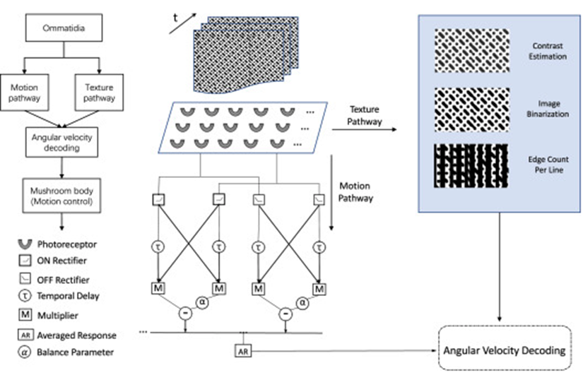
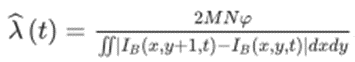
Based on the assumption that honeybees sense the complexity of textures through visual cues, such as edge orientation, size, and disruption, the texture estimation pathway is proposed to establish image contrast (H. Wang et al., 2020). Indeed, simulated input signals received by the retina are first processed by the pathway where the image contrast and spatial frequency of the grating are measured using light intensities. Specifically, the image contrast Ĉ(t) is estimated using an equation involving the highest and lowest light intensities across the visual field at a specific time t (Equation 1) (H. Wang et al., 2021). The input image is then transferred into binary image IB(t) with an intensity threshold (Equation 2) to estimate the spatial frequency λ(t). This data value is estimated by counting the number of boundary lines in the binary image across the entire visual field and is computed using Equation 3, where M and N correspond to the number of vertical and horizontal receptors in every ommatidium in a bee’s eye, and 𝝔 represents the angular separation between pixels (H. Wang et al., 2020).
Equation 1:
Ĉ(t) = (Imax(t) – Imin(t))/(Imax(t) + Imin(t))
Equation 2:
Ithreshold(t) = (Imax(t) – Imin(t))/2
Equation 3:
Furthermore, in the case of the motion detection pathway, four layers are used to examine temporal data. The first layer is that of the ommatidia, which receives the initial input image sequence. The visual information is processed by the retina, where the light intensities are captured and smoothed by ommatidia. This process can be mimicked and simulated using a Gaussian spatial filter, which is computed using Equation 4, where x, y, and t are spatial and temporal positions, I(x, y, t) is the input image sequence, and G(u, v) is a Gaussian kernel (H. Wang et al., 2020). As the visual system in the honeybee is more sensitive to intensity changes than absolute intensity, a lamina layer, which computes these intensity alterations, is used to process the input image frames. In particular, each photoreceptor calculates luminance change of pixel (x,y) at time t, L(x, y, t) using Equation 5, where H1(u) is a temporal filter, and H2(u) is the temporal filter corresponding to the persistence of the luminance change (H. Wang et al., 2020). The resulting data is used to obtain primary visual motion information. Luminance changes are then separated into on or off pathways in the on and off layer, where the on pathway processes brightness increments, while the off pathway focuses on light intensity decrements (Pinto-Texeira et al., 2018). Two processing pathways are used in the AVDM to ensure that honeybees or MAVs can efficiently navigate complex environments.
Equation 4:
P(x, y, t) = ∬I(x – u, y – v, t)G(u, v)dudv
Equation 5:
L(x, y, t) = ∫P(x, y, t – u)H1(u)du + ∫L(x, y, t – u)H2(u)du
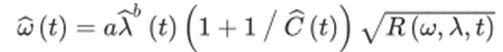
Moreover, the final layer proposed in H. Wang et al.’s (2020) AVDM is the angular velocity decoding layer, which contains multiple parallel detectors corresponding to all the visual columns in a honeybee’s ommatidia. Due to the various spatial positions of the detectors, the information yielded by these detectors differs from one another (Fu et al., 2020); therefore, the simulated model must use the diverse data received to accurately derive the angular velocity ⍵. This decoding process can be explained using an approximation method, which computes the ratio of the temporal frequency R(⍵, ƛ, t) (found using many additional equations) to the spatial frequency ƛ(t) (Equation 6) (H. Wang et al., 2020). In this complex equation, ‘a’ is a scale parameter, Ĉ(t) is the image contrast, and the parameter ‘b’ is used to tune the spatial independence. Thus, through the various formulas used to decode the angular velocity in AVDM, engineers can create functional MAVs with similar flight control to the honeybee.
Equation 6:
Automatic Terrain Following & Tunnel Centering
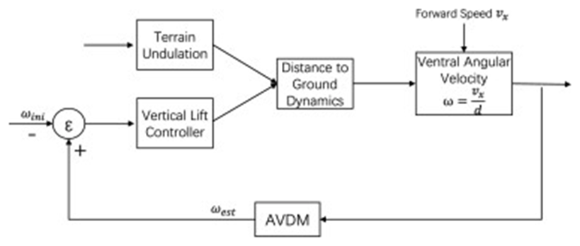
While estimating the angular velocity is essential to control a MAV’s flight, more control systems must be implemented to enable the MAV to adapt to environmental changes. Studies suggest that the honeybee adjusts its flight altitude to regulate the ventral angular velocity perceived by both its eyes to navigate safely through tunnels and tight areas (Srinivasan et al., 1996). Using this concept, developers can regulate the angular velocity to a constant value and program the MAV to alter its flight altitude depending on whether the angular velocity has increased or decreased compared to its regulated value (Figure 5) (Ruffier & Franceschini, 2015). Therefore, the AVDM can estimate the angular velocities at different spatial positions and times during the MAV’s flight, and the angular velocity regulation system can adjust the MAV’s vertical lift according to the difference between the preset angular velocity and the consecutive estimated values using artificial neural networks. This overall procedure allows the MAV to automatically follow terrain and center itself in tight areas, such as tunnels, by continuously estimating the angular velocity during its flight.
Artificial Neural Networks for Taste Reception
Taste Reception
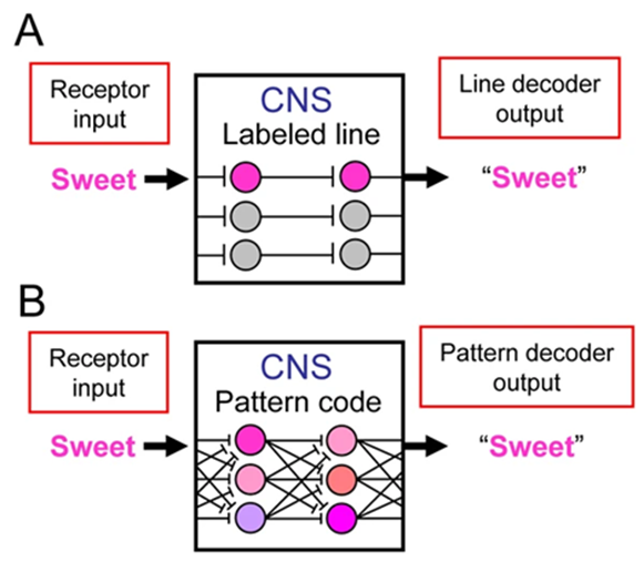
To this day, there is still debate and gaps in our knowledge on how exactly the gustatory neural circuits are organized to process the information about taste. The process begins when a taste stimulus comes in contact with a taste cell present in the taste buds (Varkevisser et al., 2001). The binding of chemical stimuli triggers many mechanisms for depolarization and the propagation of action potentials toward the gustatory afferent neurons. Usually, taste cells can be activated by more than one taste quality; where the basic tastes are considered to be: salty, sour, bitter, sweet and umami. However, it has been observed that different taste cells respond best to different stimuli – e.g. “sweet best” would respond the most to sweet stimuli – but that is not to say that they do not respond to all of them (Nagai, 2000). Gustatory neural coding is hypothesised to be the product of, one or both, of the following models: labeled-line (LL) and across-neuron/fiber pattern (ANP/AFP) (Verhagen & Scott, 2004).
Labeled line theory suggests that taste is encoded by the activation of a particular neuron or group of neurons with a similar sensitivity (Verhagen & Scott, 2004). This linear notion implies that the activation of those particular neurons only has one purpose. On the other hand, across-neuron pattern asserts that taste is coded by the pattern of activity across a neuron population (Verhagen & Scott, 2004). That is to say, input from the taste cells is distributed over multiple neurons and is associated with a pattern code in the nervous system (Figure 6). Furthermore, when studying taste reception, it is important to analyze not only the spatial aspect of neuron distribution but also the evident temporal component as well. To grasp a proper understanding of the gustatory neural circuit, one must also consider the time intervals of which the taste responses are measured. Behavioral studies conducted on rats have shown that they do not need more than 1 second following contact to respond to taste stimuli (Lemon & Katz, 2007). As such, studies must quantify the activity of gustatory neurons based on the action potential spikes measured within the first few hundred milliseconds of stimulation (Lemon & Katz, 2007).
ANN Modelling
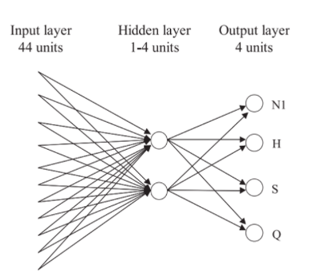
In the following study, an artificial neural network (ANN) was used to model and analyze neuron responses from the taste relay of rats. The ANN consisted of: a layer of 44 input units, a layer of hidden units, and a layer of 4 output units (Figure 7) (Verhagen & Scott, 2004). To clarify, the inputs are a representation of the 44 thalamic taste cells (Verhagen & Scott, 2004) and the output represents the basic tastes, excluding umami. Moreover, to take into account the temporal component, each 100-ms time interval was considered as a separate input unit (Verhagen & Scott, 2004). The back-propagation algorithm was used to train the model’s output to distinguish between tastes on the basis of input gathered by the neurons (Verhagen & Scott, 2004). Simply, the backpropagation is a mathematical tool that achieves desired outputs by comparing already achieved system (biological) values (Vaughan, 2015). It is used to compute derivatives and gradients organized by weights or significance (Vaughan, 2015). ANNs can use it as a learning algorithm by tuning the weights of the inputs in order to achieve the desired output (Vaughan, 2015).
After the ANN’s outputs became closer to the desired values, that is, it became more trained; the study found that the loss of just a couple of inputs that held the most significance – e.g. “sweet-best” – caused a dramatic reduction in the network’s taste distinguishing abilities (Verhagen & Scott, 2004). Thus, when analyzing the neural code pertaining to taste, it was shown that not all neurons contributed homogeneously to taste reception.
Discussion
Beyond the world of sensory processing, artificial neural networks have a multitude of other applications. For example, artificial neural networks play a significant role in character recognition and image processing. Character recognition can be used to detect handwriting, which has applications in fraud detection. Moreover, image processing can have a wide range of applications, from facial recognition in social media to cancer detection in medicine (Mahanta, 2017). Since artificial neural networks can take visual and auditory signals as inputs, they also have applications in speech recognition and language processing (Mahanta, 2017). Specifically, in the biomedical industry, artificial neural networks are just starting to be looked at for their applications in medicine and beyond. Currently, the research is mostly focused on recognizing diseases from various scans, like cardiograms, CAT scans, and ultrasonic scans (Nayak et al., 2001). As artificial neural networks learn by example, all that is needed for the network to learn and function as a disease-recognition outlet is a set of examples representing all disease variations. Then, when presented with similar-looking inputs, the network can classify the disease based on past knowledge (Nayak et al., 2001). For instance, an artificial neural network was trained to recognize the difference between the benign and malignant types of breast cancer according to nine attributes, such as clump thickness, cell size, cell shape, adhesion, bare nuclei, nucleoli, et cetera. When the trained network was tested on 239 unseen individuals, only seven of them were incorrectly predicted, showing the high accuracy of the network (Nayak et al., 2001).
Conclusion
Artificial neural networks are modelled after the brain’s interconnected neural system and are created to simulate its electrical activity using perceptron units with weighted connections. Neural networks are efficient at modelling olfactory systems for different animals. The comparable structure developed via machine learning showed a remarkably similar structure to that of the brain. This finding demonstrates how the brain is perfectly designed to process olfactory signals. Additionally, artificial neural networks can be used to mimic the vision process in animals, such as the honeybee, to allow computer-programmed machines, such as MAVs, to accurately perceive and navigate through their environment. Beyond that, ANNs can be used to help model a system, such as the gustatory neural system, and thus be able to understand the system by tuning the inputs to analyze and understand what is really going on. Applying that knowledge can aid in the manipulation, mimicking, and fine tuning of said system.
References
De Castro, F. (2009). Wiring olfaction: the cellular and molecular mechanisms that guide the development of synaptic connections from the nose to the cortex [Review]. Frontiers in Neuroscience, 3. https://doi.org/10.3389/neuro.22.004.2009
Fu, Q., Wang, H., Peng, J., & Yue, S. (2020). Improved Collision Perception Neuronal System Model With Adaptive Inhibition Mechanism and Evolutionary Learning. IEEE Access, 8, 108896-108912. https://doi.org/10.1109/ACCESS.2020.3001396
Holländer, B. (2018, August 20). Natural vs Artificial Neural Networks. Becoming Human: Artificial Intelligence. https://becominghuman.ai/natural-vs-artificial-neural-networks-9f3be2d45fdb
Kell, A. J. E., & McDermott, J. H. (2019). Deep neural network models of sensory systems: windows onto the role of task constraints. Neurobiology of Behavior, 55, 121-132. https://doi.org/https://doi.org/10.1016/j.conb.2019.02.003
Krogh, A. (2008). What are artificial neural networks? Nature Biotechnology, 26(2), 195-197. https://doi.org/10.1038/nbt1386
Lemon, C. H., & Katz, D. B. (2007). The neural processing of taste. BMC Neuroscience, 8(3), S5. https://doi.org/10.1186/1471-2202-8-S3-S5
Mahanta, J. (2017, July 10). Introduction to Neural Networks, Advantages and Applications. Towards Data Science. https://towardsdatascience.com/introduction-to-neural-networks-advantages-and-applications-96851bd1a207
Marr, B. (2018, September 24). What Are Artificial Neural Networks – A Simple Explanation For Absolutely Anyone. Forbes. https://www.forbes.com/sites/bernardmarr/2018/09/24/what-are-artificial-neural-networks-a-simple-explanation-for-absolutely-anyone/?sh=b3b33f912457
Michalowski, J. (2021, October 18). Artificial networks learn to smell like the brain. MIT News. https://news.mit.edu/2021/artificial-networks-learn-smell-like-the-brain-1018
Nagai, T. (2000). Artificial neural networks estimate the contribution of taste neurons to coding. Physiol Behav, 69(1-2), 107-113. https://doi.org/10.1016/s0031-9384(00)00194-3
Nagyfi, R. (2018, September 4). The differences between Artificial and Biological Neural Networks. Towards Data Science. https://towardsdatascience.com/the-differences-between-artificial-and-biological-neural-networks-a8b46db828b7
Nayak, R., Jain, L. C., & Ting, B. (2001). Artificial neural networks in biomedical engineering: a review. Computational Mechanics–New Frontiers for the New Millennium, 887-892.
Pinto-Teixeira, F., Koo, C., Rossi, A. M., Neriec, N., Bertet, C., Li, X., Del-Valle-Rodriguez, A., & Desplan, C. (2018). Development of Concurrent Retinotopic Maps in the Fly Motion Detection Circuit. Cell, 173(2), 485-498.e411. https://doi.org/10.1016/j.cell.2018.02.053
Rapp, H., & Nawrot, M. P. (2020). A spiking neural program for sensorimotor control during foraging in flying insects. Proceedings of the National Academy of Sciences, 117(45), 28412-28421. https://doi.org/doi:10.1073/pnas.2009821117
Ruffier, F., & Franceschini, N. (2015). Optic Flow Regulation in Unsteady Environments: A Tethered MAV Achieves Terrain Following and Targeted Landing Over a Moving Platform. Journal of Intelligent & Robotic Systems, 79(2), 275-293. https://doi.org/10.1007/s10846-014-0062-5
Sayin, S., Boehm, A. C., Kobler, J. M., De Backer, J.-F., & Grunwald Kadow, I. C. (2018). Internal State Dependent Odor Processing and Perception—The Role of Neuromodulation in the Fly Olfactory System [Review]. Frontiers in Cellular Neuroscience, 12. https://doi.org/10.3389/fncel.2018.00011
Srinivasan, M., Zhang, S., Lehrer, M., & Collett, T. (1996). Honeybee navigation en route to the goal: visual flight control and odometry. Journal of Experimental Biology, 199(1), 237-244. https://doi.org/10.1242/jeb.199.1.237
Varkevisser, B., Peterson, D., Ogura, T., & Kinnamon, S. C. (2001). Neural networks distinguish between taste qualities based on receptor cell population responses. Chem Senses, 26(5), 499-505. https://doi.org/10.1093/chemse/26.5.499
Vaughan, J. (2015, November). backpropagation algorithm. TechTarget. Retrieved November 30, 2021, from https://www.techtarget.com/searchenterpriseai/definition/backpropagation-algorithm
Verhagen, J. V., & Scott, T. R. (2004). Artificial neural network analysis of gustatory responses in the thalamic taste relay of the rat. Physiol Behav, 80(4), 499-513. https://doi.org/10.1016/j.physbeh.2003.10.005
Walczak, S., & Cerpa, N. (2003). Artificial Neural Networks. In R. A. Meyers (Ed.), Encyclopedia of Physical Science and Technology (Third Edition) (pp. 631-645). Academic Press. https://doi.org/https://doi.org/10.1016/B0-12-227410-5/00837-1
Wang, H., Fu, Q., Wang, H., Baxter, P., Peng, J., & Yue, S. (2021). A bioinspired angular velocity decoding neural network model for visually guided flights. Neural Networks, 136, 180-193. https://doi.org/https://doi.org/10.1016/j.neunet.2020.12.008
Wang, P. Y., Sun, Y., Axel, R., Abbott, L. F., & Yang, G. R. (2021). Evolving the olfactory system with machine learning. Neuron, 109(23), 3879-3892.e3875. https://doi.org/10.1016/j.neuron.2021.09.010