


ABSTRACT
Acoustic resonance is a natural phenomenon such that vibrations at specific frequencies tend to be amplified due to the natural properties of the medium through which they travel. Depending on the medium’s mechanical characteristics, different vibrational frequencies can be amplified. The biological significance of resonance comes from its ability to take advantage of mechanics to minimize the necessary energy expenditure to produce vibrations. Animals have long employed vibrations to convey or receive information, sometimes developing communication between conspecifics; information reception is essential for adaptation to changing environments. Thus, evolution has enabled species to optimize energy expense by harnessing resonance, creating biologically engineered machines known as resonating devices. Fundamentally every family in the animal kingdom employs resonance for information transfer or reception, though for exceptionally varied functions. Cicadas harness resonance for mating calls via specialized bodily features that create clicks at the natural resonant frequency of their tymbal plate, while bats, dolphins, and spiders amplify sounds for echolocation and navigation, though all through different media; bats echolocate through the air, dolphins through water, and spiders through their own silk webs. The diversity in both the users and the manifestations of resonance in the animal kingdom is astounding. This review examines resonating devices through a mathematical lens, employing frequency domain analysis and signal propagation geometry to elucidate how the mechanisms for a variety of manifestations of resonance can be represented by similar mathematical techniques. We demonstrate the use of mechanical, architectural, biomaterial, and acoustic engineering principles in the evolutionary fabrication of biological resonating devices, as well as the fundamental role of vibrations in animal behaviour and adaptability to their changing environment.
INTRODUCTION
Mathematics is often brushed over when considering the wonders of the animal world. It seems that the physical and chemical properties of an animal’s body are often the concentration of most scientific exploration. In fact, the mathematics controlling the chemistry and physics that guide the biological manifestation of animal cells, tissues, organs, appendages, and systems are rarely analyzed. This, sadly, makes sense as reaching back to every mathematical principle behind biology is exhaustive and often redundant. This is because physical and chemical models are much simpler and more effective ways of understanding the phenomena that are observed within the animal kingdom. For example, it would be arbitrarily complex to analyze the quantum mechanics of why every chemical structure exists in every report about the bone structure of antlers. Instead, more basic chemical models are sufficient to thoroughly explain these structures. However, there are many cases where these mathematical principles diffuse out into the phenomena we observe. This often reveals a much greater truth about the device itself. In other words, sometimes, we must consider these principles to fully understand a system seen in the animal world. One such example is resonating devices, where the mathematical principles are apparent in the proper functioning of these animal parts. For example, it is crucial to understand the idea of harmonics to grasp standing waves in spider webs, or the Fourier Transform to appreciate the clever design of the bat cochlea.
The following four sections will delve into different examples where a mathematical understanding is paramount to describing a resonating device’s functionality. This paper will focus primarily on signal processing and the Fourier Transform. First, the ability of spiders to process signals through the Fourier Transform and the frequency domain will be discussed. Next, the inner working of the ears of bats will be analyzed, demonstrating a mechanical application of the Fourier Transform. Further on, the principle of nonlinear signals will be introduced when talking about the cicada songs. This is because nonlinear sound signals, unlike regular linear signals, can carry more acoustic energy. Finally, the packet structure of waveforms in lion roars will be investigated.
FREQUENCY DOMAIN MODELLING OF VIBRATION IN THE SPIDER WEB
The spider web has been well-characterized as a multifunctional resonating device (Otto, Elias, & Hatton, 2018; Frohlich & Buskirk, 1982), behaving as an extended phenotype for many web-weaving Araneae (Mortimer et al., 2018). Spiders have used their webs as a means to passively ensnare prey since at least the late Carboniferous period (Garwood et al., 2016; Mariano-Martins, Hung, & Torres, 2020; Vollrath & Selden, 2007), though the web’s uses have expanded to discrete identification of prey vibrations, courtship vibrations from potential mates (Frohlich & Buskirk, 1982), and signals of avian predators (Klärner & Barth, 1982; Lohrey et al., 2009; Stafstrom et al., 2020); all while filtering out biologically irrelevant information from wind or rain (Masters, 1984, Mortimer et al., 2016). The primary method of vibration differentiation involves the use of resonance and attenuation in the web through a strategy called frequency filtering (Frohlich & Buskirk, 1982; Mortimer et al. 2013, p. 43; Mortimer et al., 2016); spiders perform frequency filtering by manually modifying mechanical properties of the web, such as web tension, geometry, and silk modulus, but also through chemical manipulation of the amino acid concentrations in their silks (Andersen, 1970; Mortimer, 2017; Su et al., 2018). These controls allow spiders to dampen frequencies indicative of environmental noise and amplify significant signals. This section examines the Frequency Based dynamic Substructuring (FBS) of the spider web to mathematically evaluate the significance of web tension, geometry, and silk composition in terms of their effects on the vibrational properties of the web. We analyze the mechanical, architectural, and acoustic engineering principles used by spiders through a mathematical lens.
Modelling using Frequency Based Dynamic Substructuring
Dynamic substructuring (DS) is the process of assembling the dynamic response of a system from the individual responses of isolated subcomponents (Otto, Elias, & Hatton, 2018). This method is often less arduous than global methods, where the entire system is analyzed at once and provides more specific information on local dynamic behaviours that may be less apparent in whole-structure analysis (Klerk, Rixen, & Voormeeren, 2008). In relation to spider webs, decomposing the system into individual silk sections and examining the local vibrational behaviours allows for modeling of the web as a resonating device, providing insight into the significance of web tension, geometry, and silk composition in the mechanical properties of the web.
DS is advantageous for modelling vibration patterns in spider webs because it can be performed in many domains, including the frequency domain (Otto, Elias, & Hatton, 2018). While most graphical representations of vibrational signals plot amplitude with respect to time (these representations are known as functions in the time domain), it is also possible to map a signal by its component frequencies. This involves decomposing a complex vibrational signal into its pure tone sinusoidal frequencies, then determining how much of the overall vibration can be attributed to each constituent pure tone. Fourier hypothesized that any vibrational signal could be constructed by superimposing different pure sinusoids, which is how frequency domain analysis was developed (Kulkarni, 2000). Figure 1 below demonstrates how a complex signal can be approximated increasingly accurately by superimposing several pure sinusoidal functions.
Using this technique, any signal, x, can be perfectly approximated by adding an infinite number of pure sinusoidal functions. If x is defined in terms of time, x=xt, Formula 1 below expresses this statement using an infinite series:
x(t)=\sum_{\mathclap{n=0}}^{\mathclap{\infty}}(a_n\cos\cos(n\omega_0t)+b_n\sin(n\omega_0t))where n=1, 2, 3 is an integer representing the number of sinusoids added and ω0 is the angular frequency such that ω0=2π/T, where T is the period of oscillation of the sinusoid (in seconds). an and bn can be expressed by Formulas 2 and 3 below:
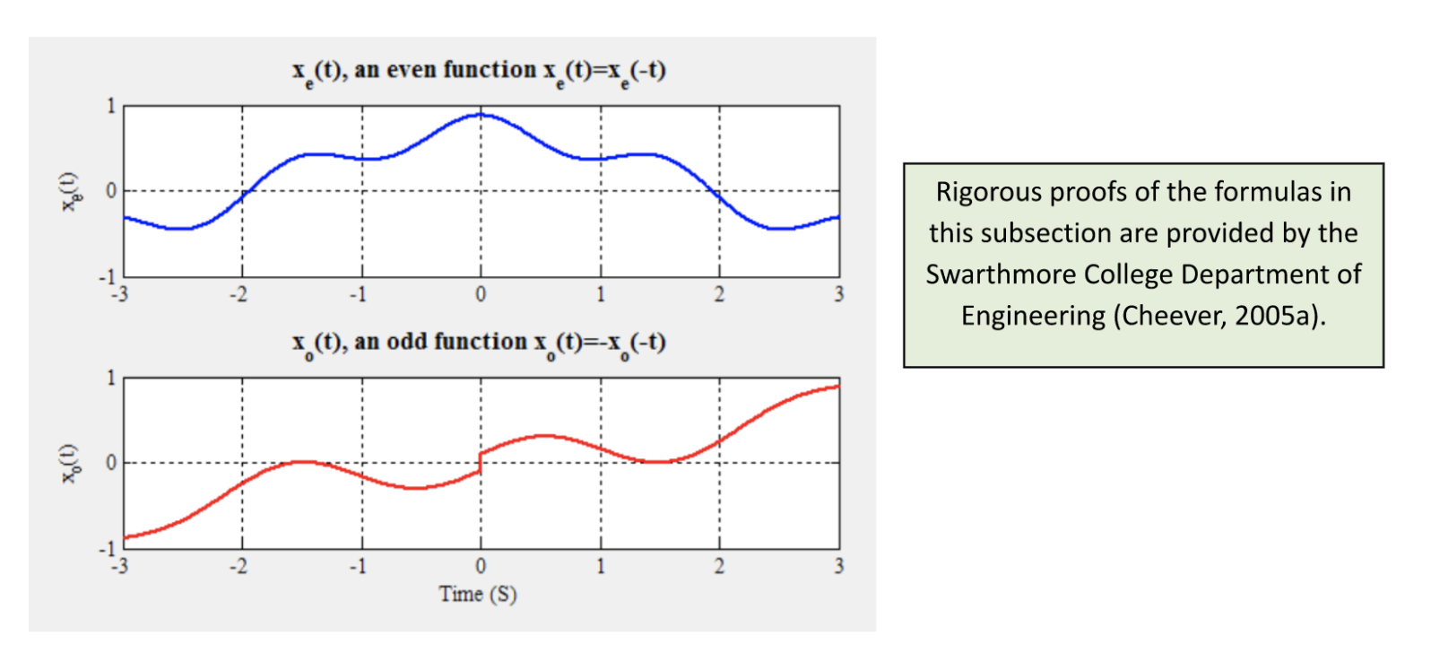
a_n=\frac{2}{T}\int_{T}x_e(t)\cos(n\omega_0t)\,dtb_n=\frac{2}{T}\int_{T}x_o(t)\sin(n\omega_0t)\,dtwhere xe(t) is the sum of even sinusoidal functions composing x, and xo(t) corresponds to all the odd functions (such that even functions are a mirror image about the y-axis, while odd functions are symmetric about the origin (Kirkpatrick, 2002); see Figure 2 below).
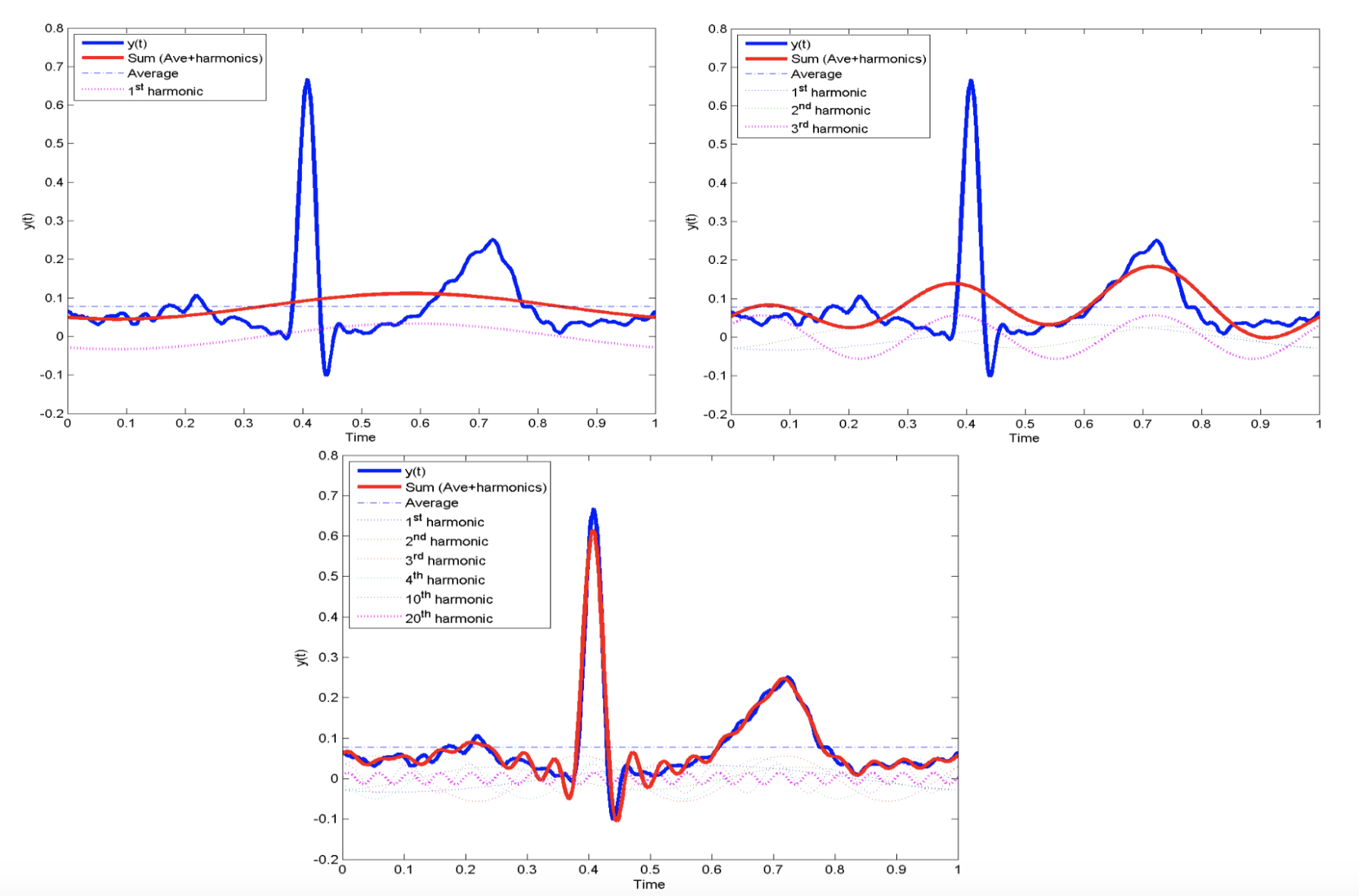
Figure 1: Approximations of a complex signal with 1, 3, and 20 pure tone sinusoidal functions. Evidently, the approximation becomes more and more accurate with more components (Cheever, 2005c).

Figure 2: Example of an even and odd complex sinusoid (Cheever, 2005a).
The expression for x(t) can be simplified using Euler’s Formula, eix=cosx+isinx (where i=√-1} ), to the following expression in Formula 4:
x(t)=\sum_{\mathclap{n=-\infty}}^{\mathclap{+\infty}}c_ne^{in\omega_0t}where cn is a coefficient dependent on n given by Formula 5 below:
c_n=\frac{1}{T}\int_Tx(t)e^{-in\omega_0t}\,dtFor cn, the product of nω0 becomes a continuous quantity (since n is any real number, -∞ ≤ n ≤+∞), so a new variable is defined: ω=nω0. If both sides of the equality in Formula 5 are multiplied to eliminate the 1/T on the right side, a new function in terms of can be defined: X(ω)=Tcn. Thus, Formula 6 illustrates the expression for X(ω):
X(\omega)=\int_{-\infty}^{+\infty}x(t)e^{-i\omega t}\,dtX(ω) is known as the Fourier Transform, which takes as input a function in the time domain, x(t), and outputs the frequency domain representation (Cheever, 2005b). Thus, X(ω) provides a method for converting a temporal function for a vibration in the spider’s web into a frequency-dependent function. Once DS has been conducted by testing the mechanical properties of the web and designing a three-dimensional model of the vibrational properties, one can use Fourier Transforms to convert time domain vibrations into frequency-dependent functions. This is essential for determining resonances in the web; frequencies corresponding to resonance frequencies will have substantially higher amplitudes than non-resonance frequencies in the frequency domain. Thus, graphical representations in the frequency domain allow for vibration amplification and attenuation intervals to be determined.
FBS Modelling for Determination of Resonance Peaks in Spider Webs
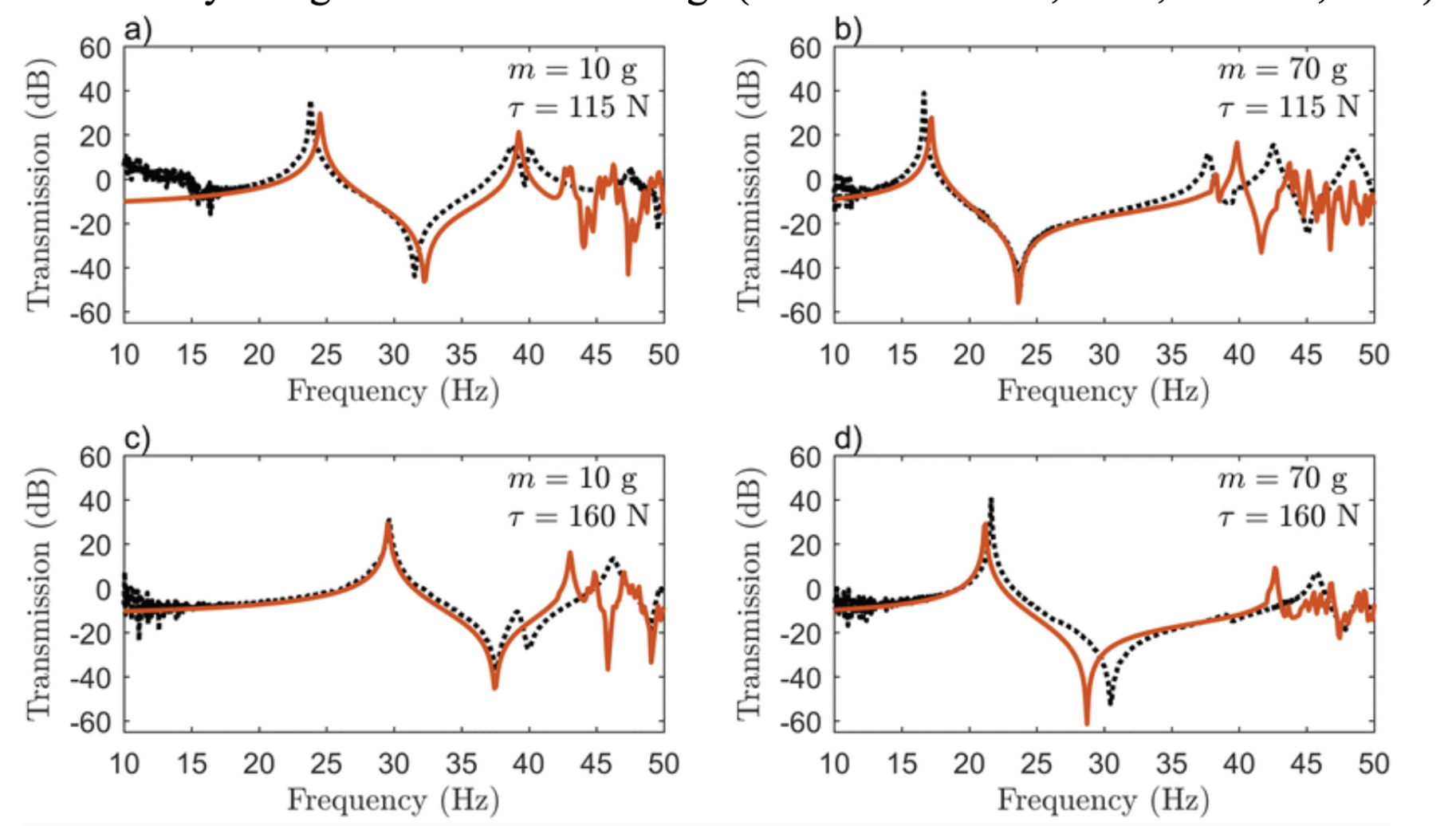
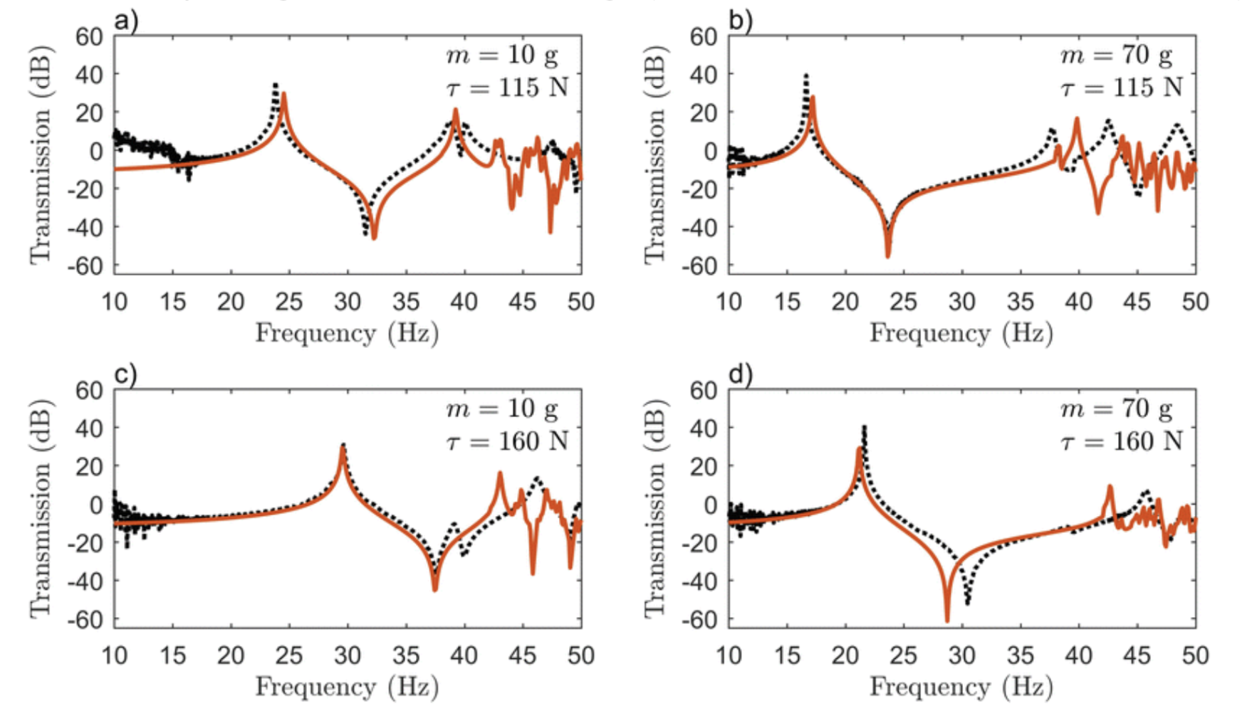
By employing the fundamentals of Fourier Transform to create an FBS model, one group accurately predicted the resonance peaks and anti-peaks for vibrations in a spider web (Otto, Elias, & Hatton, 2018). In changing the point mass applied to the web (which imitates a spider or its prey on the web) or the pretension in the silk threads, the major resonance peak shifted between 15 and 30 Hz, a doubling of its energy, major adaptability of the vibrational properties of the web (See Figure 3 below) (Otto, Elias, & Hatton, 2018). Thus, based on pretension – which the spider can modulate through active tensioning (Mortimer et al., 2016) – as well as the presence of massive objects in the web, spiders can change which frequencies are amplified and attenuated in the web. This allows for rapid adaptation to changing environmental conditions, enabling the spider to maintain the web’s frequency filtering (Mortimer et al., 2016; Naftilan, 1999). This ensures that the spider can continue to use its web as an accurate sensory mode to distinguish a variety of signals in its surroundings (Landolfa & Barth, 1996; Naftilan, 1999).
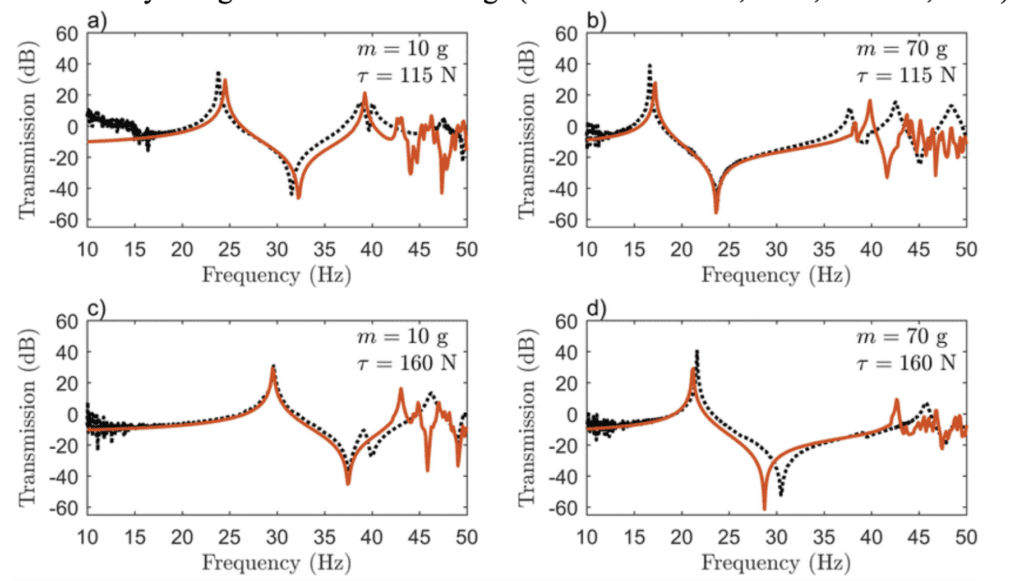
Figure 3: Model (orange) and experimental (black) frequency response for different values of the point mass (m) and radial pretension (τ) (Otto, Elias, & Hatton, 2018).
Prey ensnared in spider orb webs are predicted to vibrate at frequencies below 50 Hz (Frohlich & Buskirk, 1982), and several spider species have been observed to actively tune their webs to resonate bodies with natural frequencies in the range predicted by the FBS model (Naftilan, 1999; Parry, 1965; Watanabe, 2000). Thus, the FBS model has effectively determined the resonance peaks for orb webs, demonstrating how webs have been tailored to amplify natural frequencies commonly produced by struggling prey. However, this is not the only function of the predicted resonances. The lower end of the resonance peak is the precise frequency range used by many male species in vibrational courtship rituals (Barth et al., 1988). Most displays are species-specific low-frequency vibrations, often intermediate between background noise, like wind and rain, and prey vibrations (Barth et al., 1988). Interestingly, the natural frequency of most spiders is precisely in this range as well (Frohlich & Buskirk, 1982); this suggests that males will vibrate the webs of potential mates – usually by tugging or jerking on specific silk threads (Frohlich & Buskirk, 1982) – at a frequency that physically sways the mate in its own web (through resonance). Spiders have developed multifunctional purposes for vibrational propagation in their webs, optimizing the geometry, tension, and composition of the threads to create a sophisticated vibrational sensory mode.
Summary
Spiders use frequency filtering as a means of attenuating certain unimportant signals while amplifying vibrations indicative of ensnared prey, courtship vibrations, and avian predator calls. This section examined how the frequency domain representation of vibrations can be used in FBS to evaluate the effects of web tension, mass in the web, and architectural choice (through web geometry) on the mechanical properties of the web. The model analyzed in this section accurately determined resonances in spider orb webs, illustrating the importance of resonance for spiders for a variety of survival functions. The spider web is a sophisticated sensory mode that enables many Araneae species to perceive their surroundings through resonance and adapt to their environmental conditions.
ECHOLOCATION SIGNAL PROCESSING IN PTERONOTUS PARNELLII
Most bats have evolved a sophisticated biosonar, or echolocation, to sense their environment in low-light conditions. In echolocation, the bat emits a call, which will be reflected by objects back to the bat for signal processing. This sonar is precise enough to differentiate between target ranges with less than 0.1 mm difference or between the wing flutter of different insect species (Suga, 1990; Ulanovsky & Moss, 2008). An investigation into how bats process the reflected sound using a brain the size of a large pearl is the focus of this section and may yield interesting results applicable to sonar design.
Because bat species occupy a variety of habitats and ecological niches which demand different echolocation calls, it is difficult to offer a general model for echolocation signal processing for all bat species. Therefore, this section will focus on the mustached bat, Pteronotus parnellii. Mustached bats are long CF-FM bats, meaning that their echolocation calls are composed of a long constant-frequency (CF) portion followed by a sharply decreasing frequency modulated (FM) portion (See Figure 4 below). They are composed of 4 to 5 harmonic frequencies, with the 2nd harmonic CF component (CF2) at 61kHz being the most intense (Vater et al., 2003).
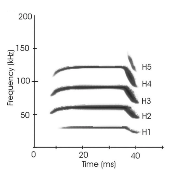
Figure 4: Echolocation call spectrogram of an adult mustached bat. H1-5 refer to harmonic frequencies. H2 has the greatest amplitude (Vater et al., 2003).
Tonotopic Arrangement of the Basilar Membrane as a Fourier Method
The first step to process sound wave data is to apply Fourier methods to change it from a function in the time domain to the frequency domain (details on Fourier analysis are given in the section on spiders). The decomposition of sounds into component frequencies occurs in the basilar membrane in the cochlea of the inner ear; it is done through physical processes, not neural computation (Brown, 2013).
A basic understanding of the cochlea is necessary to explore the function of the basilar membrane. Sound waves are transmitted to the cochlea by the stapes at the oval window. The cochlea can be simplified as a chamber filled with a fluid named endolymph. The basilar membrane lies inside the cochlea and houses hair cells which sit atop it across its length. These hair cells transform basilar membrane vibrations into nerve impulses. At the other end of the basilar membrane is the round window, which is the point at which sound waves stop propagating. Sound waves travel from the oval window to the round window, passing through the endolymph and the basilar membrane between the two, using the path of least resistance (Schnupp et al., 2011).
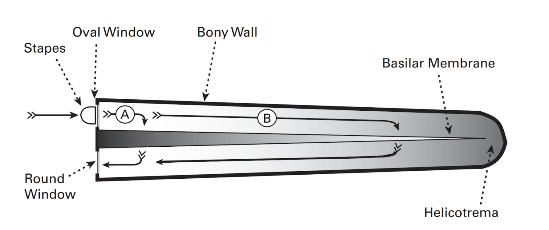
The basilar membrane has interesting mechanical properties: it is narrow and stiff at the end closest to the oval window, but wide and floppy at the other end. Thus, it offers more resistance closer to the oval window. However, the endolymph also offers resistance, as it is more difficult to displace greater volumes of liquid. The resistance of the basilar membrane and endolymph increase in opposite directions, as seen in Figure 5. Thus, sound can take a shorter path (A) to avoid the resistance of the endolymph but encounter more resistance from the basilar membrane, or a longer path (B) to avoid the resistance of the basilar membrane but encounter resistance from the endolymph. The path taken depends on sound frequency: lower frequency sounds are less affected by the endolymph resistance, and thus would take longer paths (B). Higher-frequency sounds would do the opposite (A). Thus, the basilar membrane has a tonotopic arrangement, meaning sound frequencies are distributed as a gradient along the length of the basilar membrane, with higher frequencies closer to the oval window. Each hair cell and associated nerve along the basilar membrane are thus responsible for only a small range of frequencies (Schnupp et al., 2011).

Figure 5: Simplified representation of an uncoiled cochlea. The grey shading represents resistance gradient from the basilar membrane and endolymph. Sound waves arrive from the oval window and travel through the cochlea to the round window, passing through the basilar membrane. Higher frequency sounds take a shorter path (A), while lower frequency sounds take a longer one (B) (Schnupp et al., 2011).
Information Carried by the Signal
Bats can locate and identify targets by comparing emitted and reflected signals. To start, a subject’s relative position can be determined using its range, azimuthal (horizontal) angle, and elevation. A target’s distance from the bat, or range (R), is easy to evaluate from the time delay (t) between emission and reception of the pulse (see Formula 7 below):
R=2vt
where v is the speed of sound in the air.
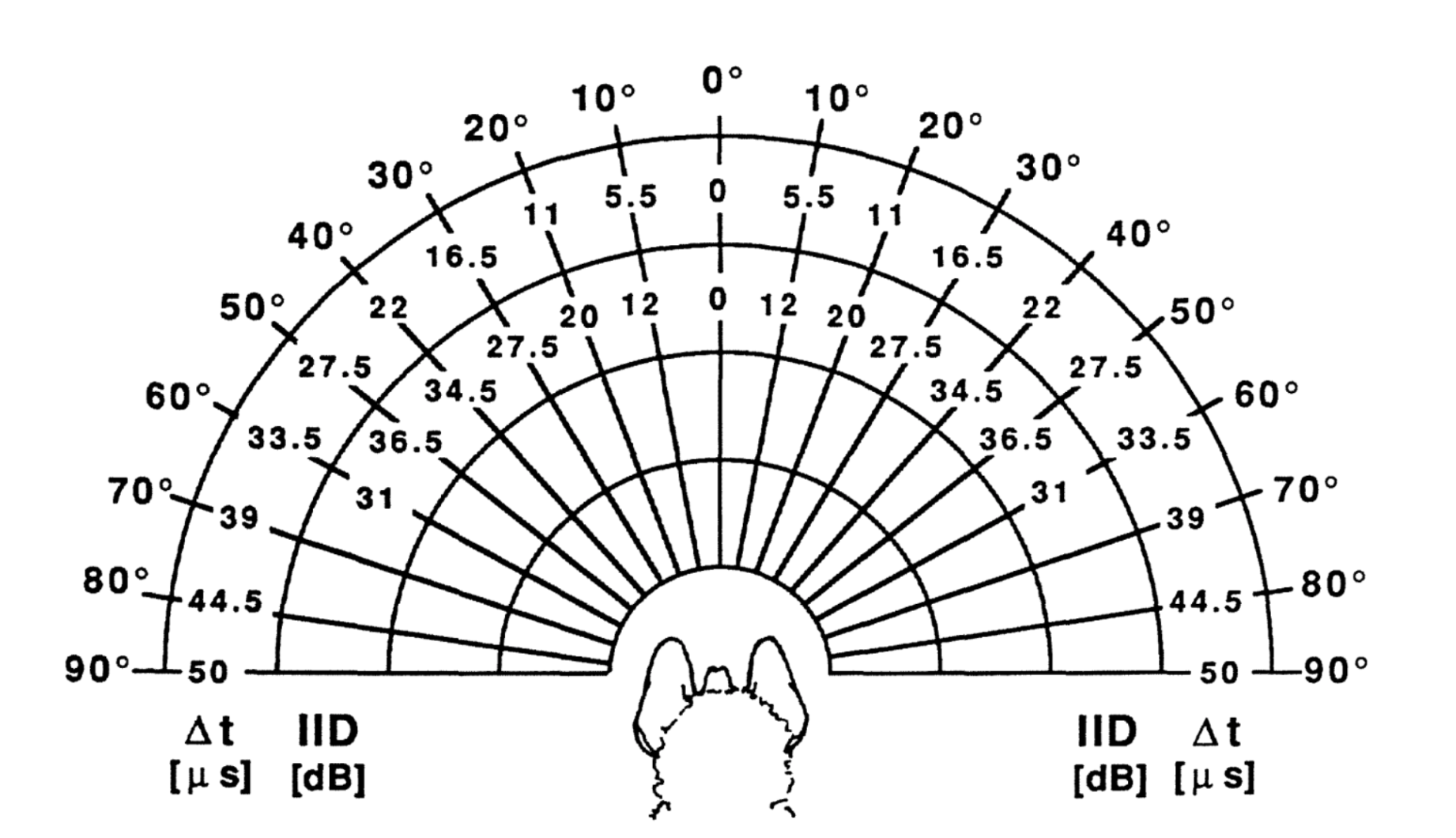
There is some debate as to whether bats use differences in time delay or intensity between the left and right ear to determine a target’s azimuth, though it is believed some combination of both is used. Because of the distance between the ears, there is a slight delay between the reception of the pulse at the left and right ear depending on the target azimuth. In addition, the shape of the head creates an acoustic shadow on one side of it, making the sound more intense in one ear than the other. These factors are illustrated in Figure 6 (Pollak & Casseday, 1989). The last factor, target altitude, can be determined from interference patterns in the echo created by the bat’s outer ear (Lawrence & Simmons, 1982).

Figure 6: Interaural time (Δt) and intensity (IID) disparities between left and right ear at various azimuthal angles around the head of a black mastiff bat (Pollak & Casseday, 1989).
Bats can also acquire specific information about targets. Indeed, different targets have different reflective and absorptive properties, shapes, and textures, which generate echoes with different spectral compositions (Pollak & Casseday, 1989). In addition, determination of target size can be achieved by analyzing the intensity of the echo. The sound intensity received by a target can be expressed as shown in Formula 8:
I=\frac{P_0}{4\pi R^2}e^{-\beta R}where I is the sound intensity (in watts/meter2), P0 is the emitted power (in watts), R is the range (in meters), and β is the atmospheric attenuation factor (in meters-1, this is a function of sound frequency, and is larger for higher frequencies).
Only a portion of the emitted power proportional to the cross-sectional area of the target will be reflected to the bat. Thus, the sound intensity received by the bat can be expressed as shown in Formula 9 below:
I=(\frac{P_0}{4\pi R^2}e^{-\beta R}=\frac{P_0\sigma}{16\pi ^2R^4}e^{-2\beta R}where σ is the acoustic cross-section of the target (in meters2).
Thus, larger targets create a higher-intensity echo, which the bat can detect (Denny, 2004).
Finally, mustached bats possess certain adaptations which allow them to detect Doppler frequency shifts in the CF portion of their calls. Indeed, the basilar membrane becomes thicker in the region around 61 kHz (CF2), and outer hair cells around this region become much more responsive, making this region more sensitive. Also, mustached bats shift the frequency of their emitted calls downwards when travelling forwards so that, after being Doppler shifted by their own movement, the emitted CF2 frequency remains around 61 kHz. This mechanism, called Doppler-shift compensation, ensures that only the movement of targets shifts the CF2 frequency. Mustached bats, then, can use these minute changes in frequency to determine target velocity and acquire enough precision to ascertain the speed of insect wing flutter (Pollak & Casseday, 1989; Ulanovsky & Moss, 2008).
Neural Signal Processing in the Auditory Cortex
After mechanotransduction in the cochlea, the signal is processed sequentially, starting at the cochlear nucleus and going through the lateral lemniscus, inferior colliculus, medial geniculate body and, finally, the auditory cortex (Suga, 1990). Interestingly, throughout most of these structures, a tonotopic organization can still be found, where frequencies are arranged spatially to different neurons (Pollak & Casseday, 1989). Additionally, different tasks in the analysis of signal data have been parceled in different parts of the auditory cortex (Suga, 1990). The Doppler-shifted constant frequency (DSCF) area, CF-CF area, and FM-FM area of the auditory cortex (shown in Figures 7 and 8) will be explored below.
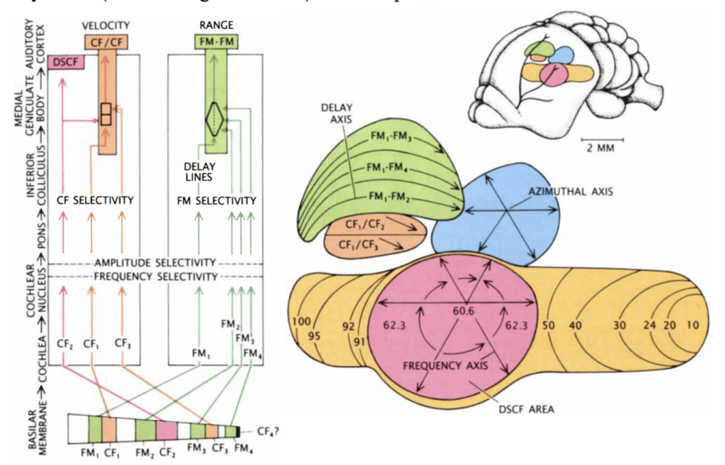
Figure 7: On the left: Different CF and FM harmonics excite different parts of the basilar membrane. The signals are sent through parallel pathways for processing. As the signals travel through the pathways, neurons become more selective for frequency and amplitude. Before the CF/CF and FM/FM areas, different pathways join for comparison in order to yield velocity and range. On the right: mustached bat auditory cortex. Different structures are coloured. Among these, the primary auditory cortex (yellow) contains the Doppler-shifted constant frequency (DSCF) area (pink). Combination-sensitive neurons are present in the FM-FM (green) and CF-CF (orange) areas (Suga, 1990).
The roughly circular DSCF area occupies 30% of the primary auditory cortex, despite only representing frequencies between 60.6 and 62.3 kHz. Here, the tonotopic organization expands to include magnitude as well. Along the surface, each neuron is coded to a specific frequency and magnitude, such that both are crudely arranged in a polar coordinate system. Relative to the center of the area, frequency increases along the radius, and amplitude changes depending on the angle. The DSCF area only detects the received CF2 pulse without comparing it to the emitted pulse and is therefore likely involved in the frequency and amplitude discrimination necessary for target identification as well as the detection of frequency changes created by flying insects. Additionally, this region is likely involved in the precision of Doppler-shift compensation (Suga, 1990).
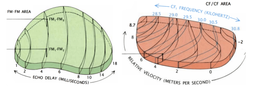
Figure 8: On the left: FM/FM area. Neurons along each black line correspond to a specific echo delay. On the right: CF/CF area. Neurons along blue lines correspond to specific CF1 frequencies combined with varying CF2 frequencies. Relative velocities were calculated, and neurons along black lines correspond to specific relative velocities (Suga, 1990).
To detect the relative velocity of targets, mustached bats must compare the CF components of their emitted pulse with the CF component of the reflected pulse. This is done in the medial geniculate body and the CF/CF area. CF1, CF2, and CF3 signals are integrated in the medial geniculate body and projected to the CF/CF area, which contains two types of neurons: CF1/CF2 neurons, and CF1/CF3 neurons. These respond strongly when the emitted CF1 component (28-30 kHz) is paired with a returning CF2 (around 61 kHz) or CF3 (around 92 kHz) component, respectively, but weakly when only one signal is present. The best combination of frequencies varies on the CF/CF area surface along two axes: the best CF1 frequency varies along one axis, and the best CF2 or CF3 frequency varies along the other. Thus, the CF/CF region is arranged in a frequency-versus-frequency coordinate system, and each position yields a certain relative velocity (Suga 1990).
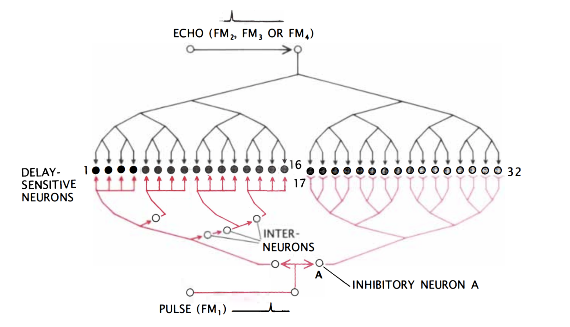
Finally, the target range is determined through the echo delay of the FM component. As in the CF/CF area, neurons in the FM/FM area respond strongly when an emitted FM1 pulse and a received FM2, FM3, or FM4 (FM2-4) are combined, but weakly otherwise. Each FM/FM neuron is tuned to a certain echo delay, and most to a certain echo amplitude as well, and they are arranged on the surface along a time delay axis. These signals are also integrated in the medial geniculate body and projected to the FM/FM area. The assignment of time delay depends on a special mechanism in the medial geniculate body (shown in Figure 9). Delay-sensitive neurons (DSNs) respond strongly when they receive FM1 and FM2-4 signals simultaneously, acting as an AND operator. On one side, the FM1 signal is delayed through delay lines, with different time delays for different DSNs. On the other side, the FM2-4 signal reaches all DSNs at the same time. Thus, when the bat emits a sound and hears itself, the FM1 signal will reach the first DSN, then move to the second and third and so on as the sound travels. The DSNs will not respond strongly, since they do not receive an FM2-4 signal. When the sound comes back to the bat, the FM1 signal will have reached an nth DSN as the FM2-4 signal reaches all DSNs at the same time. The nth DSN receives both signals, and therefore responds strongly. Each DSN, then, is associated with a certain time delay and projects its signal to the FM/FM area. The delay may be expanded through inhibitory neurons (Suga, 1990).
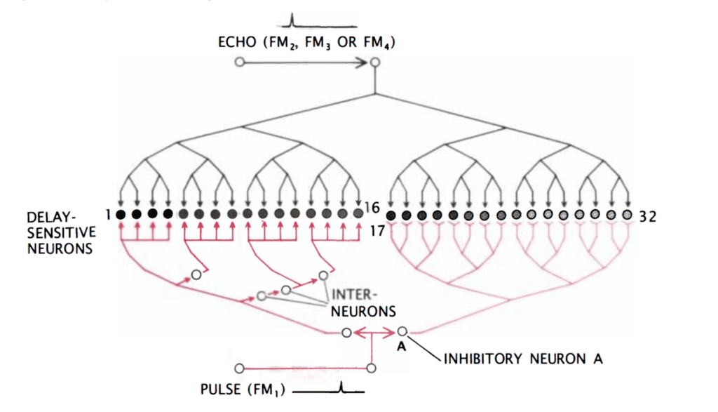
Figure 9: Model neural network in the medial geniculate body. The red portion of the network delays the FM1 signal such that the FM1 signal reaches DSN 1 first and 32 last. Inhibitory neuron A inhibits neurons 17 through 32. After some time, inhibition wears off, starting with 17, and the neurons become excited for a brief time one after the other. The FM2-4 signal, on the other hand, reaches all DSNs simultaneously (Suga, 1990).
Summary
Mustached bats use echolocation, wherein they compare an emitted sound with its echo, to acquire a surprising amount of information. The basilar membrane can be used as a Fourier method, as it employs opposing resistance from the membrane itself and endolymph to separate the sound into its component frequencies. From this signal, target range, azimuth, elevation, identity, size, relative velocity, and wing flutter speed can be determined. The signal is processed in multiple structures in the nervous system, keeping a tonotopic arrangement throughout it. Multiple areas of the auditory cortex can be separated, wherein neurons are arranged along the surface according to their frequencies or amplitudes. The DSCF area is overrepresented and contains frequencies around the CF2 (61 kHz) component to identify targets. The CF/CF area contributes to the comparison of CF signals to determine Doppler shifts and thereby determine target velocity, and the FM/FM area contributes to the comparison of FM signals to determine echo delay and thereby target range. These signals are first integrated in the medial geniculate body, which contains delay lines for echo delay determination.
MATHEMATICS OF CICADA MATING CALL AMPLIFICATION
The cicada song is iconic in many parts of the world. Perhaps this is due to its sheer volume, which is gigantic compared to the tiny size of the cicada. These intense songs are created and amplified by a tandem set of highly efficient resonators (Hughes et al., 2009; Young & Bennet-Clark, 1995). The first resonator is made up of the tymbal plate and a set of dorsal ribs. The tymbal rotates backwards and deforms the ribs successively, making an audible click (Young & Bennet-Clark, 1995). The sound waves created by the ribs match the frequency of the oscillating tymbal plate, which amplifies their sound intensity (Young & Bennet-Clark, 1995). The sound waves then exit the tymbal resonator and enter the tympana, the second resonating device. This structure acts as a Helmholtz resonator which amplifies incoming sound signals (Young & Bennet-Clark, 1995). A Helmholtz resonator is a large, hollow chamber of air with a small linear opening which simulates a spring-mass system, allowing for sound waves to be amplified.
While the resonating devices are very efficient at amplifying the clicking noise, there are surprising factors within the song’s sound propagation which help increase its volume. This is because the sound waves exiting the cicada have been shown to have nonlinear and chaotic characteristics (Edoh, 2014; Edoh et al., 2012; Hughes et al., 2009). This chaotic nature has been related to the high acoustic energy seen in cicada songs (Edoh, 2014). Before understanding why this is the case, a couple of fundamental mathematical concepts need to be defined. These will include monopole sources, dipole sources and finally, linear & non-linear signals. With these concepts understood, one can address exactly how geometric and environmental factors contribute to nonlinear sound signals, and thus, louder songs.
Geometry of Sound Sources
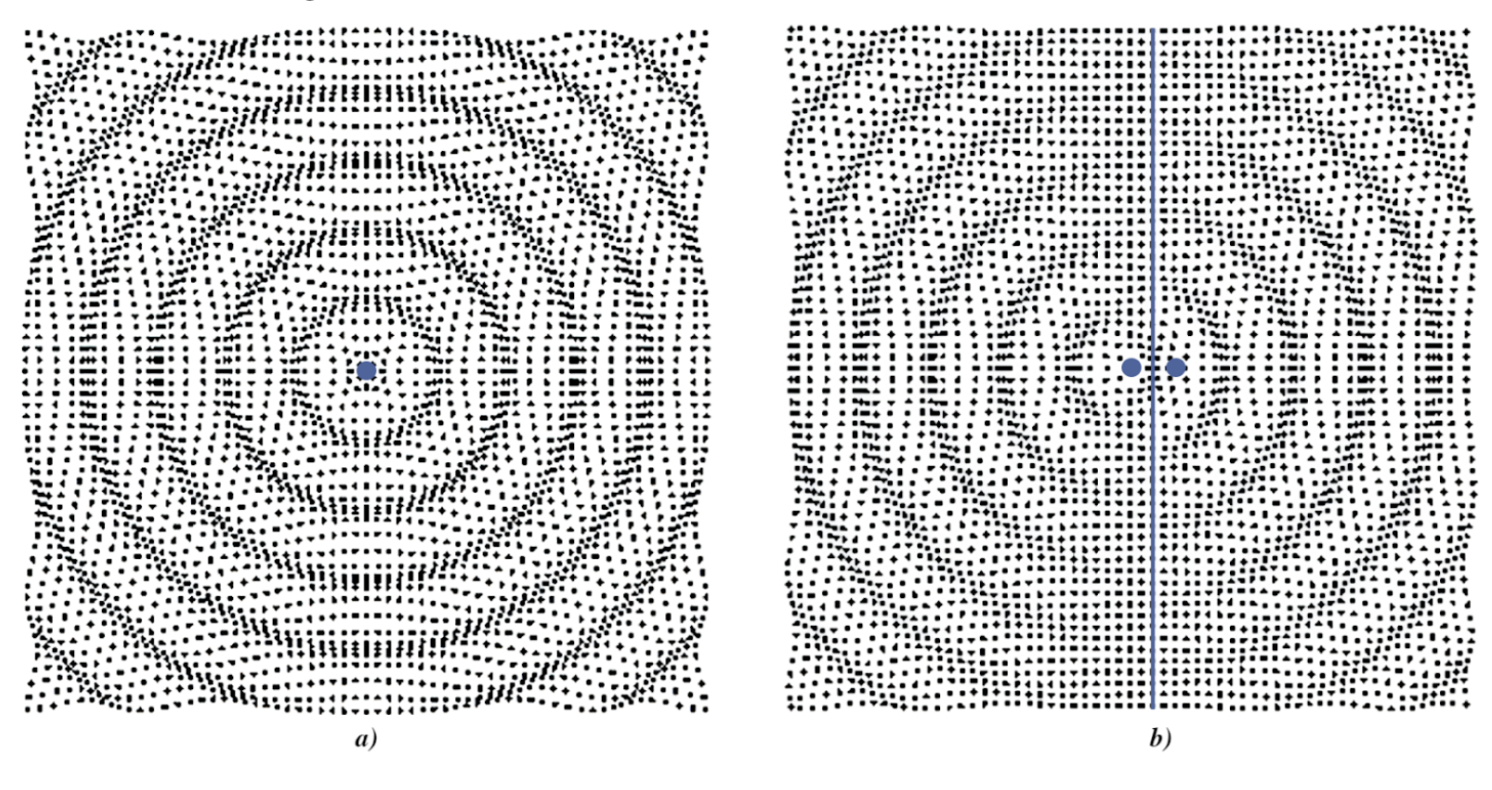
There are a few distinct models which can be used to demonstrate sound propagation around a source of audio waves. The first is a monopole source. As seen in Figure 10, a monopole source is a single point where sound waves propagate equally and spherically in all directions (Russell, 2001). The waves exiting the point source are all in phase, or in other words, the highest and lowest points of the wave signal are not shifted in time (Russell, 2001). As a result, there are no instances of constructive or destructive interference in the sound waves surrounding the monopole source. The resulting crests and troughs emanating from the source resemble the ripple effect of a pebble dropped into water. This model could be quite effective in simulating the propagation of the cicada song from very large distances, or what is known as the far-field (Michelson & Fonseca, 2000). From such a distance, the geometry of the cicada is negligible, as it simply acts as a point source.
However, from much shorter distances, these factors cannot be discounted, and a more intricate model needs to be considered. It is important to note that there are two sets of tandem resonators, with one pair found on each side of the male cicada. In other words, sound waves escape the cicada from both sides of their abdomens. With this in mind, the dipole source model seems to be a more accurate representation of the propagation of sound waves in the near field. As seen in Figure 10, the two source points emanate sound waves in opposite directions (Russell, 2001). The sound waves coming out of both sources must be out of phase due to the separation of the sources (Russell, 2001). An ideal phase shift between the two sources leads to the minimum of two bands of destructive interference, which run perpendicular to the major axis shown in Figure 10.
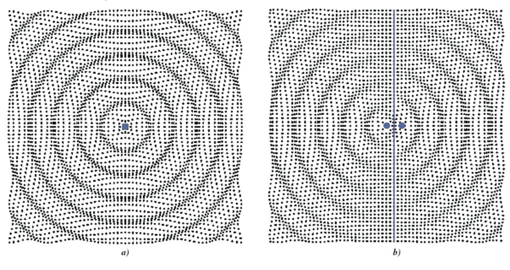
Figure 10: a) A monopole source. Waves propagate equally and spherically from a singular point source. All the waves are in phase causing a uniform wavefront. b) A dipole source. Waves propagate from two point sources spaced apart. The waves coming from each source are out of phase, causing a central axis of destructive interference (Russel, 2001).
So it would seem that from large distances, the monopole model is accurate while the dipole model is valid within very small distances. Nevertheless, there is still some more nuance that must be discussed within these models. Measurements of cicada songs have shown that sound levels are higher in regions found closer to the posterior of the cicada compared to the anterior side (Michelson & Fonseca, 2000). It is likely that the cicada’s anterior body parts block some of the sound waves, as the bulky metathorax and expansive wings can dampen the outgoing sound waves. This could help in explaining why cicadas orient themselves with their heads upwards while singing, as they have evolved to efficiently propagate their songs (Michelson & Fonseca, 2000). This means that in the far-field, the model should resemble a shielded monopole source, where certain regions in the arc of propagation have quieter sound waves. This is analogous to a speaker, which acts like a monopole, and a speaker in a cabinet, which is a shielded monopole (Russel, 2001). From this, it would seem logical that the same would be applied to the near field, where a shielded dipole model would be the most accurate in describing the sound wave propagation within short distances. While this is the case, the near field becomes far more complex as it starts to deal with nonlinear sound signals, likely because of this erratic geometry.
Linearity and Non-Linearity in Sound Signals
Linearity is a common characteristic seen in many types of mathematical systems, functions, and transforms (Smith, 1999). All of these take an input and return an output according to a specific mathematical operation. From now on, all three will be referred to by the general term function. These functions can model physical phenomena, as their inputs are measured data of a system being analyzed, and the outputs are predictions about the system. As a result, these functions are deterministic. This simply means there is direct cause and effect in the physical phenomena we study.
Linear functions are a particular subset of these deterministic models. They are simple, yet effective ways of simulating real-world systems. This is because many physical phenomena have linear characteristics, meaning linear models can represent them accurately. Additionally, their simplicity stems from the fact that linear functions are computationally friendly; they have two specific characteristics which act as mathematical shortcuts. The first characteristic is homogeneity (Smith, 1999). This is where the numerical coefficient attached to an input is not altered by the linear function in question (Smith, 1999). The definition of homogeneity is shown in Formula 10:
F(ax)=aF(x)
where F is a function which takes an input, x, and returns the output F(x).
The second characteristic of linearity is additivity (Smith, 1999). This is whenre an input with multiple terms is not altered by the linear function. In other words, the sum between the terms is preserved sinceas it is not transformed as it becomes an output (Smith 1999). The definition of additivity is shown in Formula 11:
F(x+y)=F(x)+F(y)
where F is a function which takes the input x + y and returns the output F(x + y).
These two characteristics may seem trivial, but they make these functions much simpler, which is ideal for creating models of the physical world.
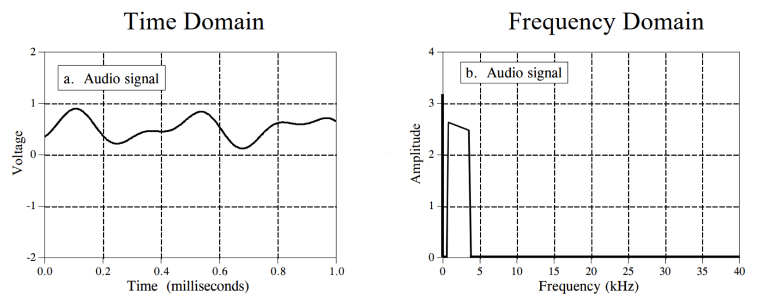
The reason why we must discuss linear functions is that they are used extensively in the world of modelling and processing sound signals (Smith, 1999). This is because any linear sound signal can be modelled as a Fourier Transform. A Fourier Transform is a function which decomposes a linear signal into a linear combination of sine and cosine waves (Smith, 1999). This is shown in Figure 11, where a linear signal is expressed as the sum of sine waves by determining what frequencies are found within the waveform. It is important to note that sine waves are also linear functions (Smith, 1999), making the entire Fourier Transform a relatively simple, yet very accurate model in the world of acoustics. For more on the Fourier Transform, refer to the Echolocation Signal Processing in Pteronotus Parnellii section of this paper.

Figure 11: A Fourier Transform finds the basis of the frequencies used within a waveform. These frequencies are visualized in the graph on the right; it shows which frequencies are dominant within the signal. From this information, we can express the original audio signal as an infinite sum of sine waves with different frequencies (Smith, 1999).
However, modelling nonlinear sound waves is a different story. Not only do they lack the computationally friendly characteristics of linear sound signals, but they are also inherently more complex as they can exhibit chaotic properties (Edoh & Hughes, 2012; Pierce, 2019; Smith, 1999). Non-linear sound signals are linear signals which have been distorted by a variety of different environmental factors (Leissing, 2006; Pierce, 2019). This could include atmospheric absorption, interference from sound waves bouncing off uneven surfaces and even meteorological effects (Leissing, 2006). Technically speaking, every sound signal is non-linear, as there is always some sort of distortion acting on the signal. However, when these distortions are negligible, signals can still be accurately modelled through linear functions and therefore classed as linear signals (Leissing, 2006; Pierce, 2019, Smith, 1999). However, when the distortions of the signal cannot be ignored, they are classed as nonlinear signals (Pierce, 2019). All sound signals are deterministic; there is a cause for every sound created. However, certain nonlinear signals can be chaotically deterministic. While chaotic determinism acknowledges cause and effect, it disregards it when it comes to practicality. A system is chaotically determinant when there are so many factors and variables at play in and around a physical system that it becomes impossible to make accurate predictions (Bishop, 2017). An example of a chaotically deterministic system is the weather on Earth. If one were to have the exact momentum and position of every air particle in the atmosphere, they could theoretically predict tomorrow’s forecast very precisely (Stevens, 2013). However, it is practically impossible to know all these factors and how they interact to influence the system being analyzed. Therefore, the system looks chaotic and random to a practical observer who can only know so many initial conditions (Bishop, 2017).
Nonlinear signals can exhibit chaos which makes their modelling a challenge for scientists and mathematicians. Despite this, there are few methods to model nonlinear signals. The first is to ignore the chaotic parts of the signal and make it resemble a linear signal (Smith, 1999). The next three methods rely on three different equations: the Burger’s equation, Fubini’s solution and the Khokhlov-Zabolotskaya-Kuznetsov (KZK) equation (Leissing, 2006). The derivations behind these equations are highly complex and not within the scope of this paper. Suffice it to say, they can help model the waveforms of nonlinear signals by accounting for the major forms of distortion, such as diffraction, atmospheric absorption and dissipation (Leissing, 2006). This helps narrow down the chaos found within the waveforms to make more coherent signals to analyze.
Why Cicadas Are So Loud
Now that we have a solid understanding of the monopole and dipole models as well as the difference between linear and nonlinear sound signals, we can model the sound propagation of the cicada song. This will help reveal exactly why the cicada song is so loud coming from such a small animal. As mentioned previously, the shielded monopole model is accurate when listening in from large distances (Michelson & Fonseca, 2000). The sound waves from this distance are linear as the distorting factors acting upon the signal are negligible (Edoh et al., 2014). These include the geometry of the cicada’s body as well as other environmental factors. However, in the near field, the shielded dipole model is the most accurate. This is because the separation between the pair of tandem resonators is not trivial, which means there will be some wave interference to consider. Furthermore, the sound waves observed near the cicada will have nonlinear and chaotic characteristics (Edoh, 2014; Edoh et al., 2012; Hugues et al., 2009). This is likely because near the sources, the geometry of the cicada (which interacts with the sound waves) as well as the diffraction and dispersion effects have a much larger impact on the sound waves (Edoh, 2014). Furthermore, the tympana resonator is believed to amplify incoming sound waves into nonlinear signals (Edoh, 2014). There is considerable evidence demonstrating that the near field is nonlinear. Edoh et al. have used the Mendousse-Burger’s equation to successfully model the nonlinear sound waves measured 15 inches away from the cicada (2012). This was then compared to actual recordings of the cicada song to check if the nonlinear equation is accurate (Edoh et al., 2012).
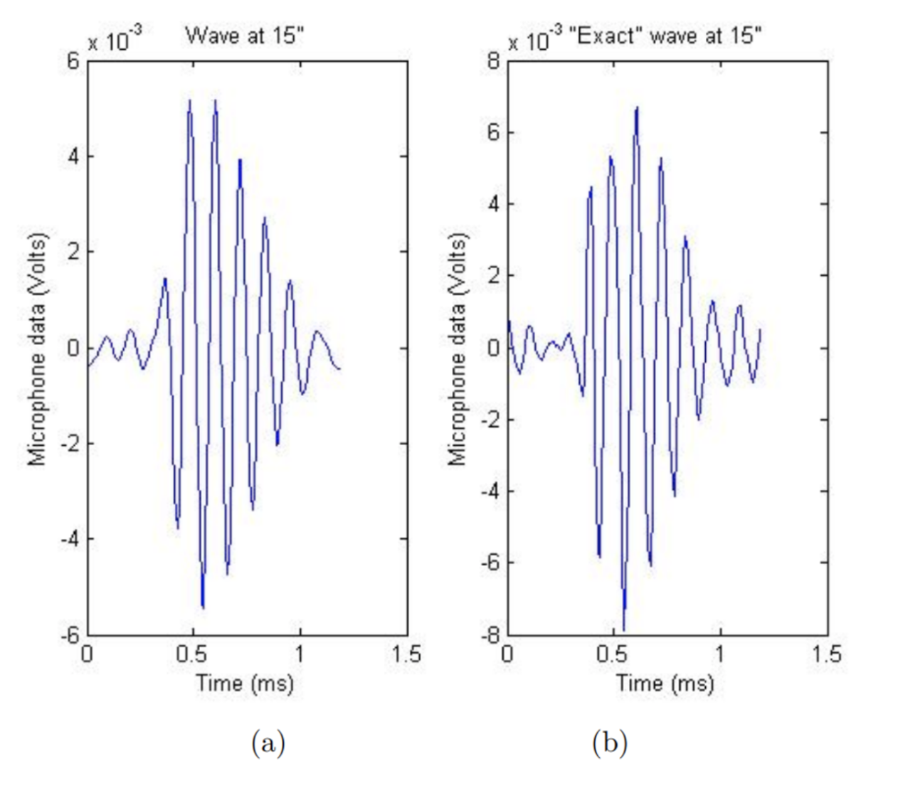
In the most comprehensive study yet, Edoh used both linear and non-linear analysis to model the far-field and near-field equations (2014). This time, both the Burger’s equation and KZK equation were compared to microphone recordings to verify nonlinearity (Edoh, 2014). See Figure 12 below.
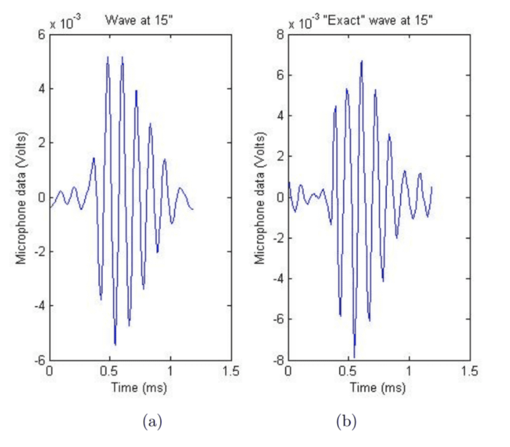
Figure 12: a) The simulated nonlinear waves computed by Edoh et al using the Burger’s equation. b) The sound wave measured by a microphone 15 inches away from the cicada. The waveformswave forms are subjectively very similar (Edoh et al., 2012).
With the cicada song now being accurately modelled, the reason why nonlinearity can contribute to the acoustic energy of the sound signals can be explained. Nonlinear signals can redistribute the energy typically found within linear signals and spread it more evenly through the waveform (Pierce, 2019). This is because the nonlinear distortions impact both the amplitude and frequency domains by adding pseudo-random spikes and dips along the waveform. This makes the signal less binary as the crests and troughs become less and less explicit. In other words, the energy of the nonlinear sound wave is spread more evenly within the wave than before, where it was concentrated within the crests and troughs. Let us not forget that the crests and troughs of linear sound waves are zones of high and low pressure propagated by the vibration of air particles. This means that the energy within these sound waves is carried through these extreme pressure zones. Researchers have found that more sound energy is found within the non-linear signals compared to the linear signals produced by the cicada (Edoh et al., 2012; Hugues et al. 2009). This is likely because the nonlinear waves carry more energy due to their chaotic nature, as well as better distributing their acoustic energy within their waveforms.
However, a question arises from this revelation. If the near field is best modelled by nonlinear waves, which are able to carry more acoustic energy, why is the song still so loud from large distances? The final key to this question comes from newer research which shows that the nonlinear sound waves reach much further than previously thought (Edoh, 2014). That is, it is more accurate to say that both linear and nonlinear waves can model the far field. Therefore, we can finally answer the question posed at the beginning of this paper: why are cicadas so loud? Cicadas can be so loud because they possess very efficient resonators. However, the propagation of the sound waves themselves also plays a major role. The nonlinear waves are seen both very close and far away from the cicada, so they can carry more acoustic energy than traditional linear waves. Thanks to these two factors, the cicada can sing incredibly loudly, considering their humble stature.
THE PROPERTIES OF PACKET STRUCTURE IN WAVEFORMS BY LION ROARING
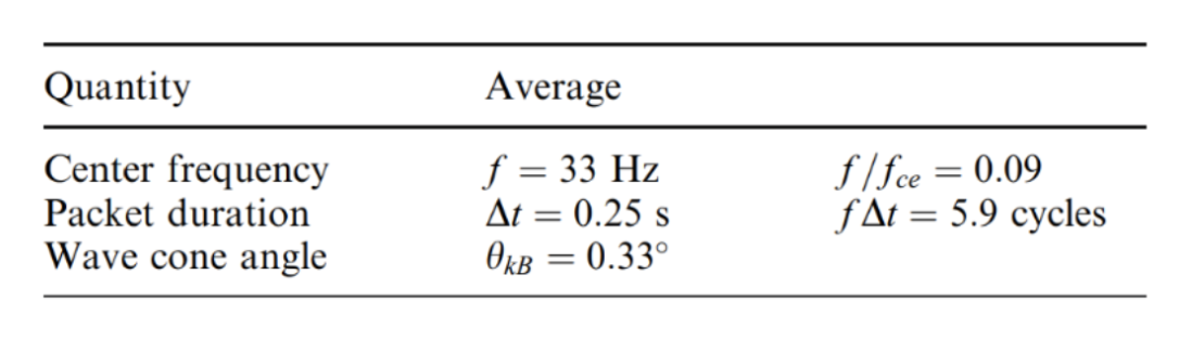
In the section on lion roars in the previously published physics paper ‘Resonating Devices In Nature For Communication And Information Reception’, the waveform formed by lion roars, which is narrow-banded, right-handed polarized waves with a typical frequency of around 120 Hz and a typical amplitude creating an equivalent magnetic field of 0.1 nanoteslas (nT) in a computer measurement was briefly introduced. This time, the properties of these packet structures of the waveform, also using the instruments mentioned in the previous section will be calculated. The instrument that detects roaring – the Equator-S magnetometer – has an average sample rate of 128 Hz (i.e., 128 samples per second) and is exceptionally sensitive for testing and recording lion roars. Fornacon et al.’s description of the Equator-S magnetic field sensor is comprehensive; it is made up of two components, each housing two three-axis fluxgate magnetometers. The main sensor is at the end of a 1.8-m boom, while the other is 50 cm farther inboard. Both the primary and redundancy units’ sensors are positioned on two sturdy booms (mentioned in ‘Resonating Devices In Nature For Communication And Information Reception’).
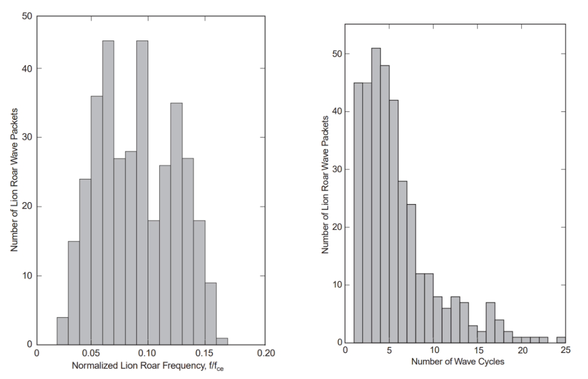
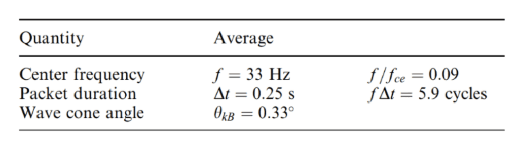
Specifically, examining the frequency and its dependency on the background field of the mirror trough, the duration of the lion roar wave packets, and the cone angle of the wave vector with the background field. The frequency distribution of lion roars, normalized to the electron gyrofrequency, fce, is depicted in Figure 13. The normalized frequencies are pretty equally distributed between 0.05≤ f/fce ≤0.15, with a mean normalized frequency close to 0.1. This diagram demonstrates that the case distribution and average value are comparable to those (Zhang et al.). Figure 14 displays the frequency distributions of the duration of lion roar wave packets in terms of wave cycles. Half of all cases have a wave packet length of fewer than five wave cycles, and around 85% have a wave packet length of less than 10 wave cycles (Baumjohann et al.).
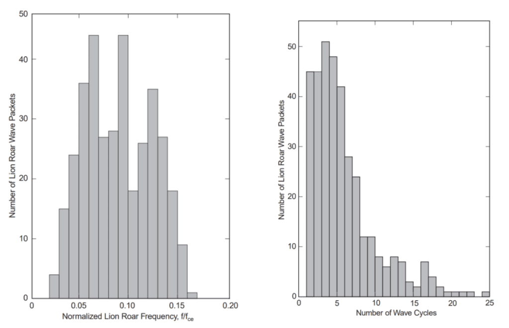
Figure 13: Occurrence distribution of normalized lion roar frequencies (left)
Figure 14: Occurrence distribution of lion roar wave packet duration (right)
As with the case studies, a minimal variance analysis was done, and the wave vector direction was compared to the direction of the ambient field. Figure 15 depicts the frequency distribution of the cone angle, θkB. Except for 10 occurrences with 1.5 ≤ θkB ≤5°, all cone angles are less than 1.4. In fact, the majority of lion roar wave packets pass over the ambient magnetic field with cone angles less than 0.2°. These values are significantly less than the usual cone angles of 10-30° (Fornacon et al.). Why? Figure 16 shows that the direction of the ambient field varies by a factor of 5-20° during a lion roar lasting several seconds. They performed a minimal variance analysis on wave packets with an average duration of 250 ms and compared the wave propagation direction to the mean of the ambient field over the same time period (Baumjohann et al.; Fornacon et al.).
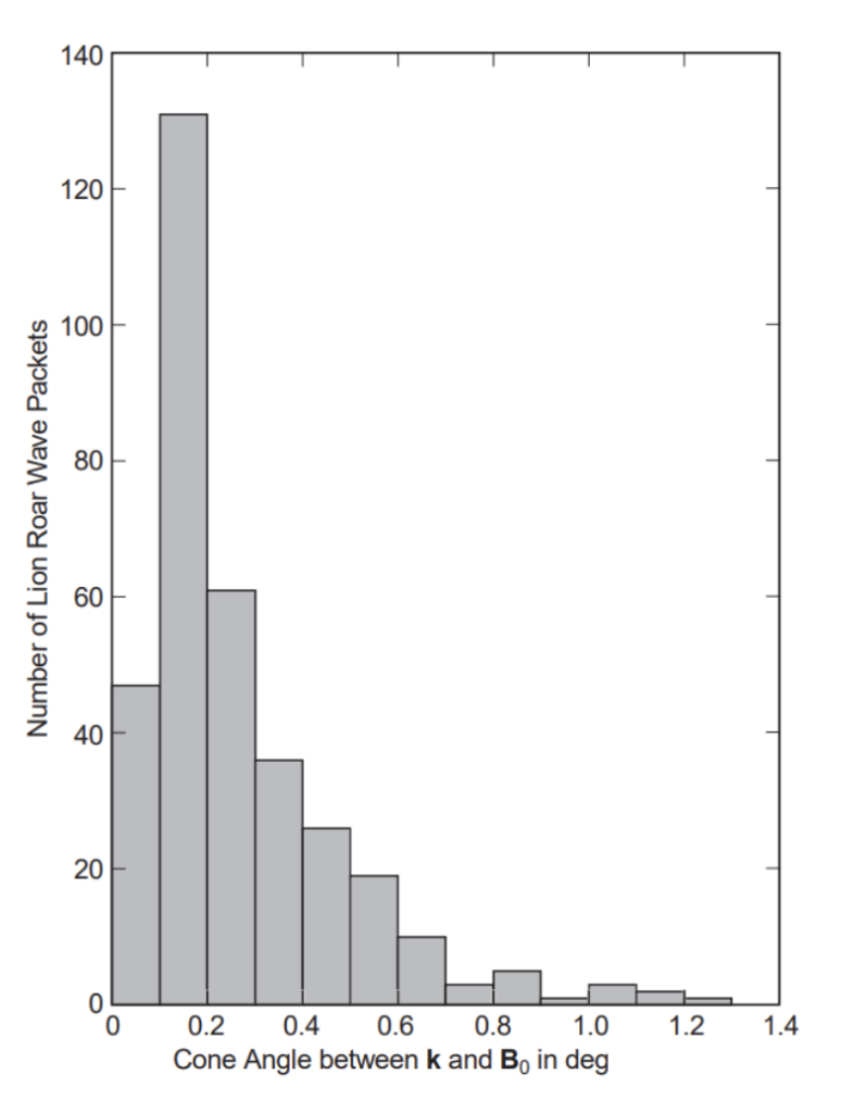
Figure 15: Occurrence distribution between lion roar wave vector and ambient magnetic field. Ten more cases (between 1.5 and 5) have been omitted from this diagram.
The signal’s narrow bandwidth is the most readily apparent feature. Since it is in the right-hand parallel whistler mode and is created within the magnetic trap configuration of the single mirror mode, the parallel whistler instability hypothesis applies (Kivelson and Southwood). Under the premise that the trapped electrons are anisotropic, dilute, and energetic enough to support the use of linear theory, the upper-frequency limit of the emission is anticipated to be as follows in Formula 12:
\frac{f_max}{f_ce}=\frac{A_e}{A_e+1}The observed values for the frequency ratio indicate that the anisotropy of the electron temperature is on the order of Ae = T⊥/T – 1≈ 0.1 for all events. On the other hand, we can benefit from the whistler resonance condition that remains true at both the upper and lower frequency limitations. We have the following formula (Formula 13):
\frac{v_{res}}{f_{ce}\lambda}=\frac{f}{f_{ce}}-1We can write this for the following limits (Formulas 14/15):
\frac{v_{min}}{\lambda_{min}}=f_{max-}f_{ce}\frac{v_{max}}{\lambda_{max}}=f_{min-}f_{ce}At the upper-frequency cut-off, the resonance condition places a lower limit on the parallel velocity of the resonating electrons (Formula 17 below):
\frac{v_{min}}{V_{Ae}}=(1-\frac{f_{max}}{f_{ce}})(\frac{f_{ce}}{f_{max}})^{\frac{1}{2}}which we estimate as v≈2.7vAe about three times the local Alven electron speed (note that the waves and particles are antiparallel for resonance).
Regarding anisotropy, the former phase is as follows (Formula 18):
\lvert\frac{v_{min}}{V_{Ae}}\rvert=\frac{A_e^{-\frac{1}{2}}}{A_e+1}Similarly, the lower frequency cut-off limits the resonant speed to its maximum value. By defining a fmin=fmax as the ratio of the measured frequency cut-offs, one obtains the frequency cut-offs ratio (Formula 19):
\frac{v_{max}}{v_{min}}=\alpha^{-\frac{1}{2}}[A_e(1-\alpha)+1]^{\frac{3}{2}}Inserting the observed values yields vmax≈1.53vmin≈4.14Ae.
According to the calculated anisotropy, the perpendicular energy E of the resonant particles is equivalent to their parallel energy, E⊥≈1.1E. EB≈(meV2Ae)/2 giving for the minimal parallel resonant energy Emin≈7.6EB and for the perpendicular energy of the resonant particles at the instability threshold yields E⊥min≈8.0EB the magnetic energy per electron. The total energy of resonant electrons at the threshold is thus Emin≈15.3EB . Proceeding along the same lines for the resonant electrons at maximum resonant energy, the numbers Emax≈17.1EB for the maximum parallel resonant energy, E⊥max≈18.8EB for the maximum perpendicular electron energy, and Emax≈36.0EB for the maximum total resonant electron energy, are obtained. These calculations demonstrate that the resonant electrons occupy a small energy range (Baumjohann et al.): 15.3≤(E/EB)≤36 with Emax/Emin≈2.35.
Figure 16 depicts the resonance zone in the v – v⊥ plane. In contrast to the vertically elongated resonant strip predicted in typical whistler resonance interaction, the resonant zone consists of a compact rectangular domain. The vertical dashed line at v=vAe is the low energy threshold limit at which positive anisotropy may initiate whistler instability. Obviously, the resonant zone is sufficiently distant from this border. Resonance is achievable only in a very restricted velocity space domain, and only a small group of electrons with almost monochromatic energy contribute to wave generation. One possible explanation is that they are the only electrons that can be captured by the wave field of the mirror. The figure’s solid lines depict the minor divergence of the electron iso-density contours from isotropy for the modest anisotropy of Ae≈0.1 . To determine if the trapping assumption is true, we may utilize the constancy of the magnetic moment μ=E⊥/B both at the highest and minimum field strengths. This results in Formula 20 below:
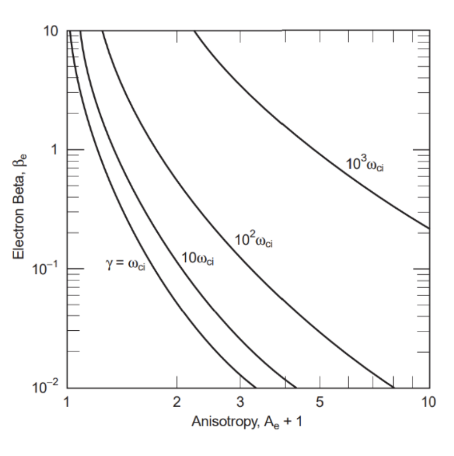
\frac{B_{max}}{B_{min}}=\frac{E}{E\perp}\approx\frac{15.3}{8}\approx2This is approximated by measurements of mirror modes for electrons reflecting near to the field maximum but still within the mirror wave bottle. The ratio of particle energy to magnetic energy per particle provides insight into the electron’s worth, since βe≈E/EB. In conjunction with the calculated anisotropy Ae≈0.1 and using the numerical solutions of the whistler dispersion relation, the maximum growth rate γ of the whistler instability in our situation is shown in Formula 21 (Gary):
\lambda max\approx10\omega\approx14\frac{rad}{s}From the whistler growth rate definition (Hasegawa) and using the value in Figure 17, Formula 22 is obtained below:
\frac{\gamma}{2\pi f_{ce}}\approx\frac{(2\pi) ^{\frac{1}{2}}n_{res}v_{Ae}}{n_0v}\left(\frac{f}{f_{ce}}\right)^{\frac{1}{2}}\left(1-\frac{f}{f_{ce}}\right)^{\frac{5}{2}}According to v≈3.5vAe, γ≈(10me)\mi = 5.4×10⁻³(for protons) and f\fce≈0.1, the fraction of resonant electrons that contributes can be obtained to calculate the properties of these packet structures of the waveform the wave growth (Formula 23):
\frac{n_{res}}{n_0}\approx0.03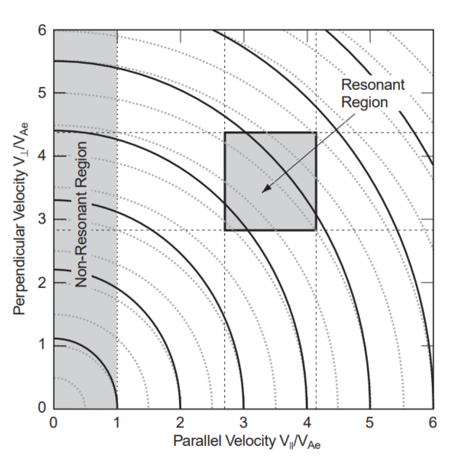
Figure 16: The resonant electron velocity space as inferred from observations. The velocities are in units of the electron Alfven velocity, VAe. The vertical dashed line at V=1 is the low energy boundary of the whistler resonance. The grey box shows the resonant region of electrons responsible for the emission of whistler waves. The solid ellipses are the iso-density contours of the weakly anisotropic electron distribution. The light circles show an isotropic distribution for comparison. Resonance takes place only in the narrow resonance region. As discussed in the text, nonlinear interaction may lead to the evolution of some residual bulge (not shown) in the resonant region which would be responsible for the observed emission (Fornacon et al.)

Figure 17 Whistler growth rates in an anisotropic electron plasma as a function of the temperature anisotropy Ae+1 and electron e (after Gary, 1993). For the measured weak anisotropy Ae=0.1 and 1 < e < 10 the growth rate is of the order of the ion cyclotron frequency γ≈ci . The curves are drawn for fpefce=100, close to that expected in the magneto sheath.
Indicating that around 3% of the total population of electrons trapped in the mirror mode bottle generates the moderate electron anisotropy that produces low frequency lion roars in the mirror modes. This study raises the question of why an extremely small number of electrons in the resonance zone is responsible for the instability of the lion roar whistlers. Without measuring the actual electron distribution function, it is difficult to address this question. Figure 16 illustrates the worldwide anisotropy of electron distribution. It shows that the wave intensities of the whistlers are rather high.
Under these conditions, electrons will diffuse from high v⊥ to high v in the resonant region. This may produce a small residual bulge on the electron distribution in the resonant strip, similar to the ion-bulge distribution predicted by Kivelson and Southwood for the nonlinear state of the mirror mode. (Kivelson and Southwood). Consequently, the distribution of primary electrons is virtually isotropic. The emission packet structure suggests that the whistler mode lion roar emissions have reached a nonlinear state. In actuality, measured amplitude translates to Formula 24 below:
E_{wB}\approx4\times10^{-13} Jm^{-3}and a whistle wave electric field represented by Formula 25:
\delta E_{we}\approx V_{Ae}\delta B_w \approx1mVm^{-1}or, a corresponding electric wave energy density represented by Formula 26:
Ew\approx\frac{\epsilon 0\lvert\delta E\rvert^2}{2}\approx5\times10^{-14}Jm^{-3}Summary
In comparison to the estimated plasma thermal energy density of nkBT ≈ 10-10 Jm-3, these figures represent fractions of 4×10⁻³ and 5×10⁻⁴, respectively. Not only would waves of this strength result in the above-mentioned quasilinear diffusion of electrons with excess perpendicular velocity towards parallel velocity, but they will also have other effects.
Inevitably, they will result in nonlinear effects such as modulational instability. Whistler wave amplitudes of 1 mV/m are quite high, on the same order as the magnetosheath’s convection electric field. It is therefore plausible to suppose that the initial excited whistlers will nonlinearly evolve into packets trapped by plasma modulations.
CONCLUSION
Despite the prevalence of physical and chemical outlooks in biology, taking a mathematical approach to describe biological processes can yield very interesting results. Multiple examples of resonating devices are explored in this paper, covering a range of uses in different contexts. Firstly, this paper examined Frequency Based Dynamic Substructuring as a model for determining the effects of web tension, mass, and geometry on the resonant properties of the web, and how these same factors are used to filter web vibrations to amplify biologically relevant signals. Then, a look into signal processing in bats was carried out, delving into the use of the basilar membrane as a Fourier method and into neural signal computation. Afterwards, the importance of nonlinear sound signals to enhance acoustic energy in cicada songs was explored. Finally, the properties of packet structures of the lion roar waveform were calculated.
Beyond the information contained within this review, some takeaways can be inferred from it as well. As tools mostly used for communication and sensation, it is unsurprising that looking at resonating devices through a mathematical lens reveals substantial information on signal processing and related topics. Relatively new concepts such as signal filtering or time domain analysis have been present in nature for millions of years, proving that much could be learned and achieved through biomimetics. In addition, the models applied here show the power of mathematical analysis in biological systems and can easily be expanded to other areas of science and engineering. As this review demonstrates, a mathematical outlook within biology should not be discounted as it can reveal information otherwise hidden to a physical or chemical outlook.
References
Andersen, S. O. (1970). Amino acid composition of spider silks. Comparative Biochemistry and Physiology, 35(3), 705-711. https://doi.org/https://doi.org/10.1016/0010-406X(70)90988-6
Barth, F. G., Bleckmann, H., Bohnenberger, J., & Seyfarth, E.-A. (1988). Spiders of the genus Cupiennius Simon 1891 (Araneae, Ctenidae). Oecologia, 77(2), 194-201. https://doi.org/10.1007/BF00379186
Baumjohann, W., et al. “Waveform and Packet Structure of Lion Roars.” Annales Geophysicae, vol. 17, no. 12, 31 Dec. 1999, pp. 1528–1534, 10.1007/s00585-999-1528-9.
Bishop, R. (2017). Chaos. In E. N. Zalta (Ed.), The Stanford Encyclopedia of Philosophy. Metaphysics Research Lab, Stanford University. plato.stanford.edu/entries/chaos/#NonDyn
Brown, C. (2013). Hair Cells [Lecture Recording]. MIT OpenCourseWare. https://ocw.mit.edu/courses/9-04-sensory-systems-fall-2013/resources/lec-15-hair-cells/
Cheever, Erik (2005). Derivation of Fourier Series. Swarthmore Department of Engineering, Linear Physical Systems Analysis. https://lpsa.swarthmore.edu/Fourier/Series/DerFS.html
Cheever, Erik (2005). Introduction to the Fourier Transform. Swarthmore Department of Engineering, Linear Physical Systems Analysis. https://lpsa.swarthmore.edu/Fourier/Xforms/FXformIntro.html
Cheever, Erik (2005). The Fourier Series. Swarthmore Department of Engineering, Linear Physical Systems Analysis. https://lpsa.swarthmore.edu/Fourier/Series/WhyFS.html
Denny, M. (2004). The physics of bat echolocation: signal processing techniques. American Journal of Physics, 72(12).
Edoh, K. (2014). Modeling Cicada Sound Production and Propagation. Journal of Biological Systems, 22(4), 617-630. doi.org/10.1142/S0218339014500235
Edoh, K., Hughes, D., Katz, R. (2012). Nonlinearity In Sound Signals. Journal of Biological Systems, 21(1). doi.org/10.1142/S0218339013500046
Fornacon, K.-H., et al. “The Magnetic Field Experiment Onboard Equator-S and Its Scientific Possibilities.” Annales Geophysicae, vol. 17, no. 12, 31 Dec. 1999, pp. 1521–1527, 10.1007/s00585-999-1521-3. Accessed 26 Nov. 2022.
Frohlich, C., & Buskirk, R. E. (1982). Transmission and attenuation of vibration in orb spider webs. Journal of Theoretical Biology, 95(1), 13-36. https://doi.org/https://doi.org/10.1016/0022-5193(82)90284-3
Garwood, R. J., Dunlop, J. A., Selden, P. A., Spencer, A. R., Atwood, R. C., Vo, N. T., & Drakopoulos, M. (2016). Almost a spider: a 305-million-year-old fossil arachnid and spider origins. Proceedings. Biological sciences, 283(1827), 20160125. https://doi.org/10.1098/rspb.2016.0125
Gary, S. Peter. Theory of Space Plasma Microinstabilities. Cambridge University Press, Cambridge, Cambridge University Press, 1993, www.cambridge.org/core/books/theory-of-space-plasma-microinstabilities/11F0E1BEEFCC3A1597230DAF2DD664F7. Accessed 26 Nov. 2022.
Hasegawa, Akira. Plasma Instabilities and Nonlinear Effects. Physics and Chemistry in Space, Berlin, Heidelberg, Springer Berlin Heidelberg, 1975. Accessed 26 Nov. 2022.
Hughes, D. R., Nuttall, A. H., Katz, R. A., Carter, G. C. (2009). Nonlinear acoustics in cicada mating calls enhance sound propagation. Journal of the Acoustical Society of America, 125(2), 958-967. doi.org/10.1121/1.3050258
Kirkpatrick C. (2002). Nelson advanced functions & introductory calculus. Nelson Thomson Learning. https://teachers.wrdsb.ca/ruhnke/files/2017/09/Nelson-Advanced-Functions-12-Textbook.pdf
Kivelson, Margaret Galland, and David J. Southwood. “Mirror Instability II: The Mechanism of Nonlinear Saturation.” Journal of Geophysical Research: Space Physics, vol. 101, no. A8, 1 Aug. 1996, pp. 17365–17371, 10.1029/96ja01407. Accessed 26 Nov. 2022.
Klärner, D., & Barth, F. G. (1982). Vibratory signals and prey capture in orb-weaving spiders (Zygiella x-notata, Nephila clavipes; Araneidae). Journal of comparative physiology, 148(4), 445-455. https://doi.org/10.1007/BF00619783
Klerk, D. d., Rixen, D. J., & Voormeeren, S. N. (2008). General Framework for Dynamic Substructuring: History, Review and Classification of Techniques. AIAA Journal, 46(5), 1169-1181. https://doi.org/10.2514/1.33274
Kulkarni, S.R. (2000). Chapter 4: Frequency Domain and Fourier Transforms. Princeton University Department of Electrical Engineering. https://www.princeton.edu/~cuff/ele201/kulkarni_text/frequency.pdf
Landolfa, M. A.; Barth, F. G. (1996). Vibrations in the orb web of the spider Nephila clavipes: cues for discrimination and orientation. Journal of Comparative Physiology A, 179 (4), 493-508. DOI: 10.1007/BF00192316.
Lawrence, B. D., & Simmons, J. A. (1982). Echolocation in bats: the external ear and perception of the vertical positions of targets. Science, 218(4571), 481–483.
Leissing, T. (2006). Nonlinear outdoor sound propagation [Master’s Thesis, Chalmers University of Technology]. Chalmers Research Portal. publications.lib.chalmers.se/records/fulltext/61697.pdf
Lohrey, A. K., Clark, D. L., Gordon, S. D., & Uetz, G. W. (2009). Antipredator responses of wolf spiders (Araneae: Lycosidae) to sensory cues representing an avian predator. Animal Behaviour, 77(4), 813-821. https://doi.org/https://doi.org/10.1016/j.anbehav.2008.12.025
Mariano-Martins, P., Lo-Man-Hung, N., & Torres, T. T. (2020). Evolution of Spiders and Silk Spinning: Mini Review of the Morphology, Evolution, and Development of Spiders’ Spinnerets [Mini Review]. Frontiers in Ecology and Evolution, 8. https://doi.org/10.3389/fevo.2020.00109
Masters, W. M. (1984). Vibrations in the Orbwebs of Nuctenea sclopetaria (Araneidae): I. Transmission through the Web. Behavioral Ecology and Sociobiology, 15(3), 207–215. http://www.jstor.org/stable/4599721
Michelson, A. & Fonseca, P. (2000). Spherical sound radiation patterns of singing cicadas, Tymanistalna gastrica. Journal of Comparative Physiology A – Sensory Neural and Behavioral Physiology, 186(2), 163-168. doi.org/10.1007/s003590050016
Mortimer, B. (2017). Biotremology: Do physical constraints limit the propagation of vibrational information? Animal Behaviour, 130, 165-174. https://doi.org/https://doi.org/10.1016/j.anbehav.2017.06.015
Mortimer, B., Gordon, S., Drodge, D., Siviour, C., Windmill, J., Holland, C., and Vollrath, F. (2013). Sonic Properties of Silks. XIV International Conference on Invertebrate Sound and Vibration [Conference notes]. University of Strathclyde, Glasgow. http://www.isv2013.org/ISV_files/ISV2013%20Abstract%20Book%20Final_web.pdf
Mortimer, B., Soler, A., Siviour, C. R., & Vollrath, F. (2018). Remote monitoring of vibrational information in spider webs. Die Naturwissenschaften, 105(5-6), 37. https://doi.org/10.1007/s00114-018-1561-1
Mortimer, B., Soler, A., Siviour, C. R., Zaera, R., & Vollrath, F. (2016). Tuning the instrument: sonic properties in the spider’s web. Journal of the Royal Society, Interface, 13(122), 20160341. https://doi.org/10.1098/rsif.2016.0341
Naftilan, S. A. (1999). Transmission of vibrations in funnel and sheet spider webs. International Journal of Biological Macromolecules, 24(2), 289-293. https://doi.org/https://doi.org/10.1016/S0141-8130(98)00092-0
Otto, A. W., Elias, D. O., & Hatton, R. L. (2018). Modeling Transverse Vibration in Spider Webs Using Frequency-Based Dynamic Substructuring. Dynamics of Coupled Structures, Conference Proceedings of the Society for Experimental Mechanics Series. Springer, Cham. https://doi.org/10.1007/978-3-319-74654-8_12
Pierce, A. D. (2019). Nonlinear Effects in Sound Propagation. Acoustics – An Introduction to Its Physical Principles and Applications (pp. 649-709). Springer, Cham.
Pollak, G. D., & Casseday, J. H. (1989). The neural basis of echolocation in bats (Ser. Zoophysiology, v. 25). Springer-Verlag.
Russell, D. (2001). Sound Field Radiated by Simple Sources. Acoustic and Vibration Animations – Pennsylvania State University. http://www.acs.psu.edu/drussell/demos/rad2/mdq.html
Schnupp, J., Nelken, I., & King, A. (2011). Auditory neuroscience: making sense of sound. MIT Press.
Smith, Edward J., and Bruce T. Tsurutani. “Magnetosheath Lion Roars.” Journal of Geophysical Research, vol. 81, no. 13, 1 May 1976, pp. 2261–2266, 10.1029/ja081i013p02261.
Smith, S. A. (1999). The Scientist & Engineer’s Guide to Digital Signal Processing. California Technical Publishing.
Stafstrom, J. A., Menda, G., Nitzany, E. I., Hebets, E. A., & Hoy, R. R. (2020). Ogre-Faced, Net-Casting Spiders Use Auditory Cues to Detect Airborne Prey. Current biology : CB, 30(24), 5033–5039.e3. https://doi.org/10.1016/j.cub.2020.09.048
Stevens, M. [Vsauce]. (2013, May 20). If [Video]. Youtube. youtu.be/QBK3QpQVnaw
Su, I., Qin, Z., Saraceno, T., Krell, A., Mühlethaler, R., Bisshop, A., & Buehler, M. J. (2018). Imaging and analysis of a three-dimensional spider web architecture. Journal of The Royal Society Interface, 15(146), 20180193. https://doi.org/doi:10.1098/rsif.2018.0193
Suga, N. (1990). Biosonar and neural computation in bats. Scientific American, 262(6), 60–71.
Ulanovsky, N., & Moss, C. F. (2008). What the bat’s voice tells the bat’s brain. Proceedings of the National Academy of Sciences of the United States of America, 105(25), 8491–8498.
Vater, M., Kossl, M., Foeller, E., Coro, F., Mora, E., & Russell, I. J. (2003). Development of echolocation calls in the mustached bat, pteronotus parnellii. Journal of Neurophysiology, 90(4).
Vollrath, F., & Selden, P. (2007). The Role of Behavior in the Evolution of Spiders, Silks, and Webs. Annual Review of Ecology, Evolution, and Systematics, 38(1), 819-846. https://doi.org/10.1146/annurev.ecolsys.37.091305.110221
Watanabe T. (2000). Web tuning of an orb-web spider, Octonoba sybotides, regulates prey-catching behaviour. Proceedings. Biological sciences, 267(1443), 565–569. https://doi.org/10.1098/rspb.2000.1038
Young, D. & Bennet-Clark, H. C. (1995). The role of the timbal in cicada sound production. Journal of Experimental Biology, 198(4), 1001-1019. doi.org/10.1242/jeb.198.4.1001Zhang, Y., et al. “Lion Roars in the Magnetosheath: The Geotail Observations.” Journal of Geophysical Research: Space Physics, vol. 103, no. A3, 1 Mar. 1998, pp. 4615–4626, 10.1029/97ja02519. Accessed 30 Jan. 2021.