


Abstract
The world of mathematics holds much value when it comes to computing, establishing, and resolving the many different complex relationships found in natural sciences. This, naturally, holds true for biological systems and their vast array of unique biomechanical tools and even for the complex diversity in social behaviors. In this paper, different modelling techniques will be used to explain the efficient aerodynamic design of avian tails numerically and to describe the clever utilization of hydrodynamic forces by aquatic tails. Additionally, the unique avian tail of the peacock, despite its limited flying capabilities, is also characterized by an energetically efficient design which can be properly understood through the concept of resonance and game theory. As a uniquely interesting example of an avian tail, it will also be treated in one of the text’s sections.
Introduction
The mathematical modeling of physical principles allows a better understanding of natural phenomena. It is also quite powerful to better grasp the mechanisms in animal life. Animal tails create an interesting scope to examine these principles, as they have a vast number of different functions and behaviors across species due to different adaptations. For this investigation, both avian and aquatic tails are discussed, as the methods that they use to interact with their environment have a variety of different effects and relationships.
This paper will first seek to demonstrate how the fundamental role of caudal fins for propulsion and steering in water can be modeled. This section aims to review the process of observing caudal fin propulsion variables and how they can be modeled and applied to robotic vehicles. Afterward, the study of movement will be dealt with by looking at the role of avian tails as they pertain to lift and drag in the atmosphere. Finally, the specific case study of the peacock tail, which comprises the sexually selected properties of both visual and auditory stimuli will serve as a conclusion.
Modeling of Caudal Fin Propulsion
Underwater vehicles are important for discovering the unknown marine ecosystem. These devices have gained inspiration from organisms that have evolved over millions of years to efficiently navigate an aquatic environment. How have aquatic organisms’ propulsive behaviors and characteristics been observed and quantified for applications in man-made devices?
The propulsive motion of fish is surprisingly complicated, and therefore, the relationship of many variables with propulsive efficiency has been observed and quantified. The main variables at play are the stiffness of the caudal region, the area of the fin, the fin strip movement, and the swing phase of the caudal movement.
Simulating Flexural Stiffness in Caudal Fin Propulsion
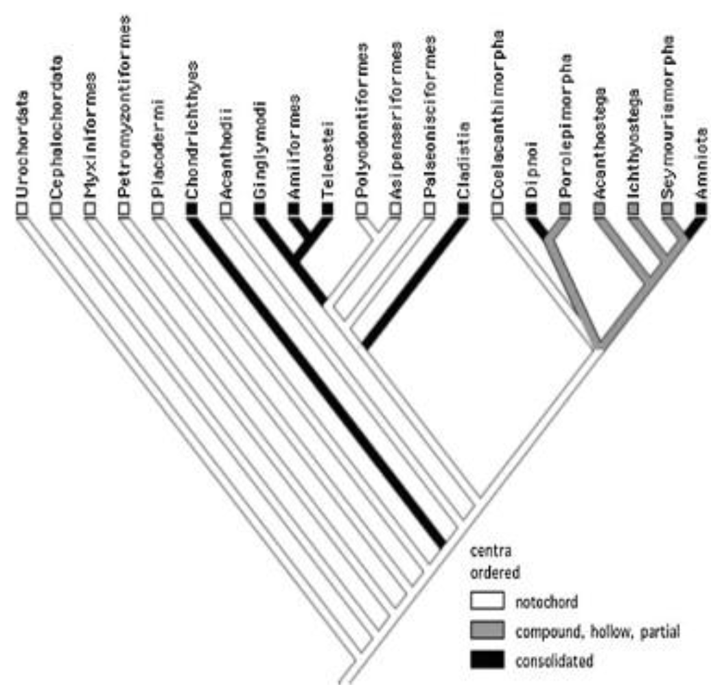
This section will provide an example of how one of the key variables in fish propulsion can be studied for optimized behavior. The study of how backbone stiffness affects propulsion is valuable due to the divergent evolution of various aquatic species. Figure 1 shows the divergent evolution of aquatic species in three separate categories: solid backbones, compound and hollow/partial backbones, and notochords (Root & Liew, 2014). A notochord is a predecessor to a spine, consisting of a continuous cartilaginous rod.

Figure 1: Fish phylogeny; note the divergence from notochord into both solid and partial backbones (Root & Liew 2014).
Root & Liew (2014) investigated the connection between flexural stiffness and propulsion through a digital animat and determined a design’s efficiency by its ability to catch prey. Figure 2A shows the structure and layout of the digital animat that they used. The animat is a plastic basin with a propulsion system made of a keel and a tail. The “eye” is light-sensing and unaligned with the axis of symmetry. The mechanism that oscillates the tail is a servomotor, an electrical device capable of precise rotation. There is also a control device that bases the turning angle of the tail on the light intensity. The animat is able to move in two dimensions and navigates on the surface of the water.
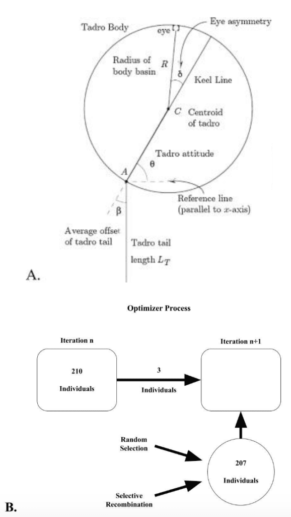
Figure 2: (A) View from above of the object whose mechanics is modeled in the simulation. (B) Flow diagram for the genetic algorithm (Adapted from Root & Liew, 2014).
After constructing and defining this animat, Root & Liew (2014) conducted a multigenerational simulation. The layout was that the best-performing individuals of a generation were carried into the next generation. Additionally, the new generation was also composed of random selection – individuals with a randomly selected set of traits – and selective recombination – individuals with the traits from two successful individuals combined in a unique manner. This selection method is shown in Figure 2B, where the population was set at 210. These conditions created a study where the evolutionary behavior of tail stiffness could be observed, where the characteristic driving stiffness was propulsive efficiency, indicated by prey-catching success.
The simulation had 5 input parameters: tail stiffness, tailbeat frequency, initial velocity, and heading. Additionally, the measure of merit (i.e., prey-catching success) is shown below as Equation 1.
\begin{equation}
MoM=\frac{1}{distance}+\frac{1}{energy+capture}
\end{equation}
In Equation 1, distance is the distance covered during the simulation, energy is the energy used while pursuing the prey, and capture is a bonus rewarded if the prey is captured. Therefore, individuals receive better scores if they are faster (less distance) and more efficient (less energy).
Figure 3 shows the results of one run of the simulation, while Figure 4 shows the stiffness values throughout the simulation, and Figure 5 shows the tailbeat frequency data across generations of the simulation.
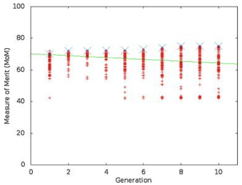
Figure 3: A view of the range of MoM values for one trial over 10 generations. The line connects the best individual in each generation (Root & Liew, 2014).
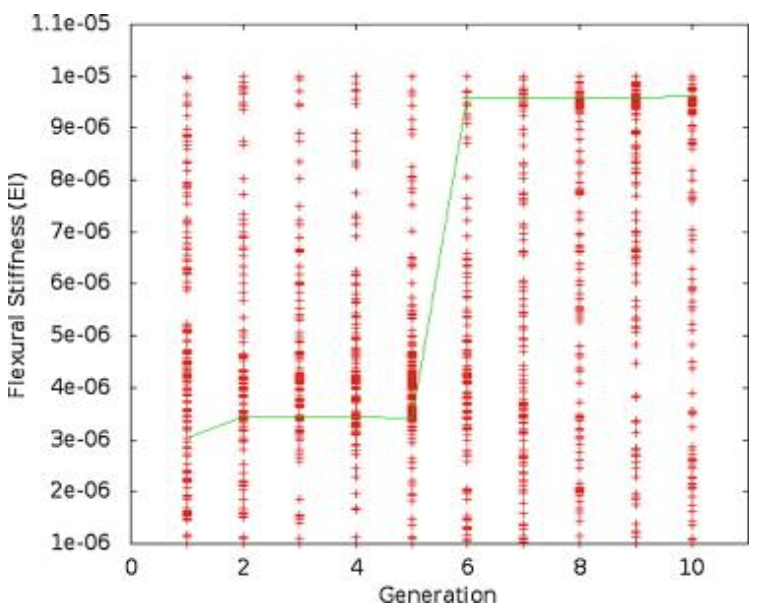
Figure 4: A plot of the flexural stiffness data for one trial over 10 generations. The line connects the best individual in each generation (Root & Liew, 2014).
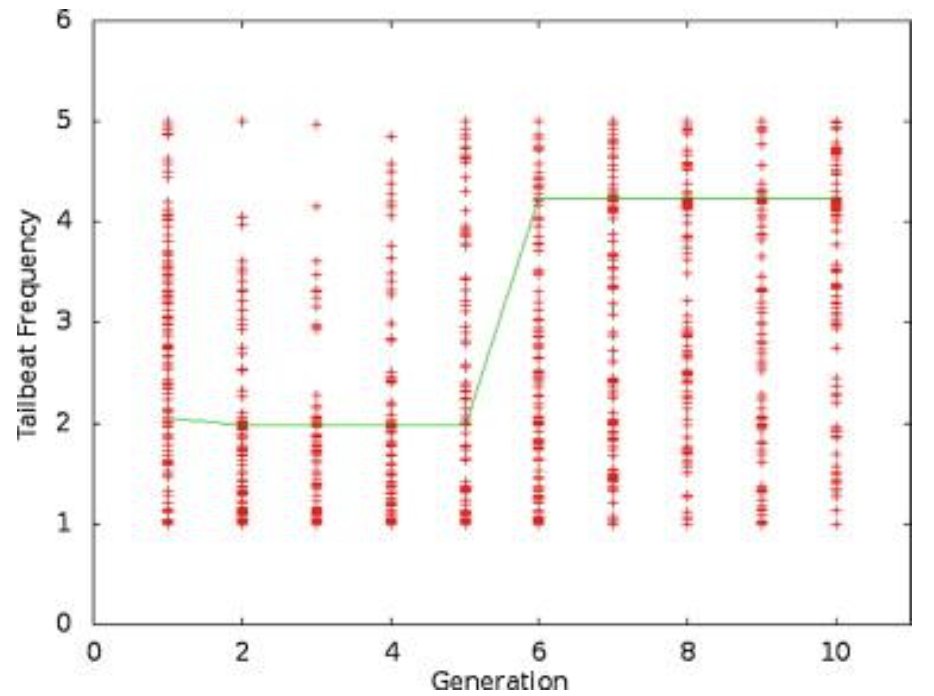
Figure 5: A plot of the tailbeat frequency data for one trial over 10 generations. The line connects the best individual in each generation (Root & Liew, 2014).
Looking purely at the raw data, there does not appear to be any trend for stiffness or frequency values across generations. However, the green line in each plot represents the best configuration in each generation, and therefore, flexural stiffness and tailbeat frequency increase across generations. It was found that in each trial performed, the majority of this increase occurs within generations 4 to 6. In the data from the provided trial, shown in Figures 4 and 5, the increase occurs from generation 5 to 6. Also, in every case, the tailbeat frequency and flexural stiffness increase simultaneously. An increase in both values indicates an increase in overall thrust (Root & Liew, 2014).
This overview of the modeling procedure performed by Root & Liew provides an example of how a variable affecting fish propulsion can be quantified through an optimization method.
Determining Efficiency of a Robotic Fish Model
Now that the study of variables to determine their ideal value for biomimetic designs has been discussed, the next subject becomes how to determine the efficiency of a created model. Wen et al. tackle this problem while mentioning that this tactic has not been recognized before.
The efficiency of a propulsive model is quantified through thrust efficiency, which is measured through undulatory power consumed by the fluid, the thrust force, and the swimming speed (Wen et al., 2012). Power consumption in robotic devices is measured by subtracting the total power from the total power consumed by the motors while they operate the undulatory movement (Wen et al., 2012). High-resolution digital particle image velocimetry (DPIV) is a method that can be used to measure the thrust force with the 2D wake around the fish.
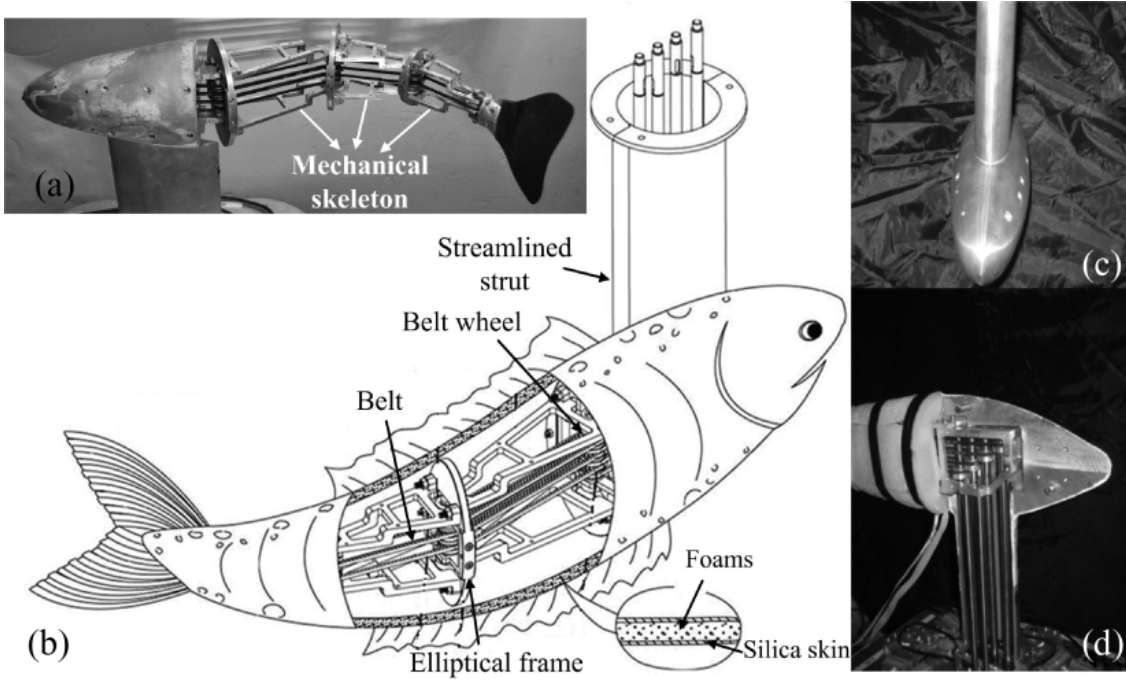
The robotic model, based on the mackerel (Scomber scrombrus), used by Wen et al. is shown in Figure 6. Figure 1a shows the sectioned nature of the model so that the undulatory movements are better at approximating the actual movement behavior of the fish.

Figure 6: (a) the structure of the robotic mackerel, (b) actuation mechanisms that rotate the robotic links (Adapted from Wen et al., 2012).
Wen et al. conducted the data analysis of their experiment using the Strouhal number, which is a dimensionless value that acts as a parameter of fish locomotion (Triantafyllou et al. 2000). It is a function of the amplitude of undulation of the caudal fin, towing speed, and flapping frequency.
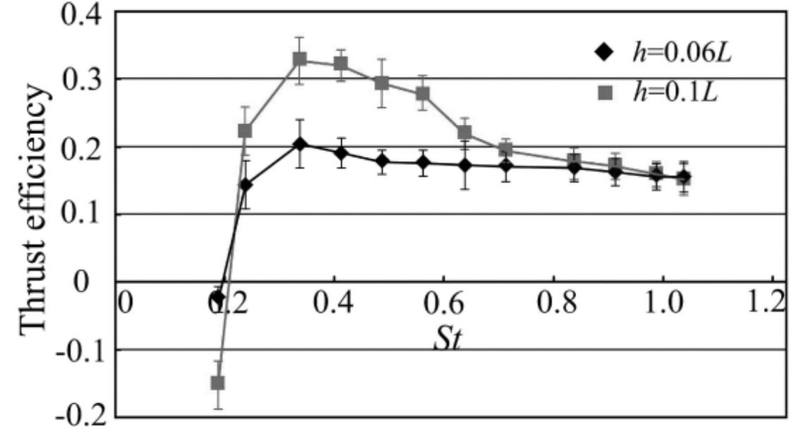
Figure 7 shows the summary of the results from Wen et al. 2012 through a plot of thrust efficiency vs. Strouhal number. These results show that the model has the greatest thrust efficiency for 0.3 ≤ St ≤ 0.325. This means that larger amplitudes are more efficient, aligning with the results of Read et al. studying the infinite flapping foil (Read et al., 2003).

Figure 7: Thrust efficiency versus various Strouhal number values for two different amplitudes (h) (Wen et al. 2012).
Concluding Caudal Fin Propulsion Modeling
The process of robotic fish creation involves two important steps: observing and quantifying the propulsive behaviors of the fish, and once a model has been created, the assessment of its efficiency. This process is important to enhance current underwater vehicle design efficiency.
Modeling Bird Tails Through Slender Lifting Surface Theory
Like aquatic animals, avian animals use their tails to help navigate through a fluid, the atmosphere. Though a bird’s flight is mostly credited to its wings, the aerodynamic functions of a bird’s tail play an important role in breaking and steering. Morphologically, a bird’s tail is situated at its rear and composed of an interlocking microstructure of feathers called the rectrices (Thompson, 2014) – this structure spans many different shapes and sizes. A 2-dimensional conception of this appendage, as well as its acting forces, has allowed scientists to model equations to define tail efficiency and the factors surrounding aerodynamic optimization.
Forces Acting on the Tail
Before the peak performance conditions can be defined, it is essential to understand the two forces acting on and generated by a bird’s tail and its rectrices: lift and drag. A bird’s tail can be assimilated to a rudder that breaks and steers upwards, downwards, to the left and right.
In a 1993 article, Thomas established that Slender Lifting Surface Theory or Slender Wing Theory, can be effectively used to model the forces produced by a bird’s tail. In this model the tail is conceptualized as a delta-shaped (meaning thin, flat, and triangular) wing of low aspect ratio AR at an angle of attack α. (Usherwood et al., 2020) – This model is only valid for an angle of attack small enough to prevent leading edge separation. The aspect ratio is a fundamental part of this model and is defined in dimensionless form as:
\begin{equation}
AR=\frac{Span_{wing}}{Area_{wing}}
\end{equation}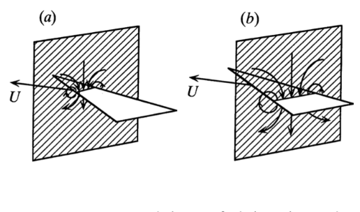
This model is particularly effective because of the tails signature low aspect ratio, allowing the flow to be defined in a two-dimensional plane (Thomas, 1993). More specifically, Thomas’s model consists of setting the flow in a two-dimensional plane, “normal to the direction of movement of the tail at a distance x from its apex.” As shown in Figure 8, the movement and velocity of the slice of tail produces a downward flow.This unsteady downstream flow is explained by two-dimensional flow theory. (Cousteix, 2003) When the tail is “pushed” further into the plane (or when the distance x from the apex is increased), while the direction of airflow remains the same, the scale of the slice of the tail present in the plane becomes greater, and therefore the scale of the flow increases. An increase in scale signifies an acceleration of mass in airflow. (Thomas, 1993). This explains the following equation for lift force:
\begin{equation}
L=U\alpha \ast\frac{dm'}{dt}
\end{equation}
Indeed, the lift force can be defined as the product of the velocity of the slice of tail with respect to its angle Uα and of the rate of increase of the local added mass m with respect to time. This equation can be further developed to depend on displacement rather than time. Since velocity is equal to the rate of change of the position, Equation 4 is obtained:
\begin{equation}
L=U\alpha\ast\frac{dm'}{dx}\ast\frac{dx}{dt}=U^2\alpha\ast\frac{dm'}{dx}
\end{equation}
Lastly, using two-dimensional flow theory’s definition of the rate of change of mass (5) and (6), an equation for lift force can be established with respect to air density ρ, and wingspan bmax ( bmax is used due to the lift depending on the widest portion on the bird tail) (7):
\begin{equation}
dm=\frac{pi}{4}pb^2dx
\end{equation}
\begin{equation}
\frac{dm'}{dx}=\pi\frac{b}{2}\rho\frac{db}{dx}
\end{equation}\begin{equation}
L=\frac{\pi}{4}\rho \alpha U^2b^2_{max}
\end{equation}As stated, a bird’s tail also produces drag. The two types of drag are induced drag (“part of the drag on an airfoil that arises from the development of lift”) and profile drag (composed of the drag caused by skin friction and the drag caused by pressure)(Oxford languages, nd). The induced drag depends on the potential flow (a term used to describe a flow using streamlines) at the widest point (Collins dictionary, nd).
As induced drag arises “from the development of lift,” it is proportional to the lift force with its equation given by:
\begin{equation}
D_i=\frac{1}{2}L\alpha
\end{equation}
Profile drag is composed of skin friction drag and pressure drag. However, in this model, neglecting pressure drag has no impact on the outcome of calculations. Following its conditions the pressure drag is identical to induced drag differentiating itself solely after the flow has separated (Thomas, 1993). Therefore, profile drag is equal to skin friction drag, leading to the following equation where S represents the surface and CDf represents the coefficient of skin friction drag:
\begin{equation}
D_p=D_f=\frac{1}{2}\rho U^2SC_{D_f}
\end{equation}
\begin{equation}
C_{D_f}=\frac{0.074}{\sqrt[5]{RE}}
\end{equation}Finally, it is well established that the coefficients of lift and drag are equal to the quotient of the force and the dynamic pressure multiplied by the surface. Therefore, the coefficients of lift and drag can respectively be given by Equations 11 and 12:
\begin{equation}
C_L=\frac{\pi}{2}AR\alpha
\end{equation}
\begin{equation}
C_{D_i}=C_l\frac{\alpha}{2}
\end{equation}To determine aerodynamic efficiency, we need to focus on coefficients as they provide a ratio with the fluid where the body is in motion. The bigger a coefficient of lift, the more aerodynamic the bird tail.
Determining Tail Morphology for Peak Performance
As per Equations 11 and 12, defined through the slender lifting surface model, at a set angle of attack, the forces generated by the tail depend strictly on the components of the aspect ratio AR of a bird’s tail: tail width (defining lift, moment, and induced drag) and tail area (determining profile drag). Using this model, conclusions can be drawn about the efficiency of morphological structures. Indeed, the higher the angle of spread of a tail, the greater its area and maximum continuous width. As seen in Figure 9, the growth rate of the tail area augments at a considerably slower rate than the maximum continuous width when the tail spread degree increases. Therefore, the greater the tail spread the greater the aspect ratio and the greater the lift and drag coefficients. Furthermore, as per Equations 11 and 12, the greater the angle of attack the greater the coefficients of lift and drag. It has been defined that “just over 120-degrees gives the best aerodynamic performance, and this may be close to a universal optimum, in terms of aerodynamic efficiency” (Thomas, 1993).
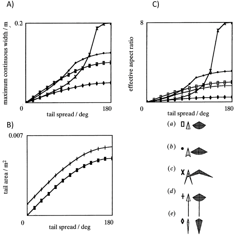
Figure 9: Graphical representation of tail maximal continuous span and area with respect to tail spread A) Maximum continuous width with respect to tail spread in degrees B) Tail area with respect to tail spread in degrees C) Aspect ratio with respect to tail spread in degrees (Thomas, 1993).
Therefore, according to this model, tail shape plays a role in performance (See Figure 10).
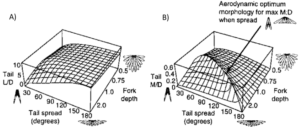
Figure 10. Graphical representation of correlation between aerodynamic efficiency and tail morphology A) Lift-to-drag ratio with respect to tail spread in degrees and fork depth B) Moment-to-drag ratio with respect to tail spread in degrees and fork depth (Thomas, 1997).
Effect Of Leading-Edge Vortices On Rotation
During flight, a bird’s entire body and tail produce three different airflow directions: streamlines, downwash and upwash (see Figure 11).

Figure 11: Representation of directional airflow generated by a gliding bird in flight (Thomas, 1993).
At high speeds, most of the lift is produced by the outermost rectrices of a bird’s tail. This produces two powerful adjacent vortices interacting with each other.
To steer, a bird can rotate its tail feathers laterally to create an asymmetry in the vortices and generate a large rolling moment and sideways force. These vortices can be visualized in our previously established 2-dimensional plane model. Indeed, in mathematics, a vortex (see streamlines in Figure 11) is defined as an area with flow revolving around a singular axis. Applied to physics, a vortex is “a mass of air or water that spins around very fast and pulls objects into its empty centre” (Cambridge dictionary).
However, assuming a given tail shape, these air vortices will become unstable if the tail is at an angle exceeding 40° with the apex (Thomas, 1993) – “Though the angle of attack at which these vortices appear [should depend] on the slenderness of a tail” (Filippone, 1999-2003). If the aspect ratio of the tail is inferior to 1, the leading-edge vortices will naturally become asymmetrical and induce rolling and rotational force on the bird’s tail. The result is a loss of control by a full rotation or simply an oscillatory motion. If the aspect ratio of the tail is superior to 1, the vortices will burst, resulting in the tail being limited to the properties of a high aspect ratio wing (Thomas, 1993).
The Visual and Auditory Stimuli From the Peacock’s Tail
Honesty of Signals
Displays of courtship often rely on the stimulation of multiple different senses and, by researching these displays, the evolutionary patterns of diversification in sexual traits can be better understood. Indeed, it is important to figure out the energetic costs, muscle power limits, and biomechanical constraints involved in these displays to evaluate what exactly they are meant to signal to their receiver. In the case of the Indian peafowl, the male peacock (Fig 1.) courts the female peahen by raising his tail and train feathers and vibrating those feathers in front of the peahen. This rattling attracts the female’s attention and always precedes copulation. Interestingly, the frequency of sound produced by the rattling is significantly correlated with the animal’s morphology. For example, train length has a high correlation with train mass and, since heavier trains require more effort to vibrate their feathers at specific frequencies and amplitudes, individuals with longer and heavier trains would be expected to produce vibrations at lower frequencies to minimize the energetic cost. However, after observing the relationship between train length and the frequency of sound produced, it was found that the opposite was true, higher frequency sounds would come from longer trains (Figure 12) (Dakin et al., 2016).

Figure 12: Image of a peacock (top) (Mitchell, 2022). Vibration frequencies during displays in relation to (A) sex, age, and (B) other factors that predict feather vibration frequencies in adult males. (A) Displaying peafowl vibrate their feathers at frequencies ranging from 22 to 30 Hz, with broad overlap in the ranges of frequencies used by different sex and age classes (Dakin et al., 2016).
Indeed, this finding shows that having a larger train does not restrict the peacock’s ability to perform sounds and vibrations at lower frequencies. Furthermore, given the previously established correlation between train length and train mass, this information suggests that longer-trained males perform displays that require greater power and energy. Conversely, it was also found that the longer trains did not have a correlation with mating success but did have a correlation with fat reserves, which would allow for greater energy expenditure and circulating androgen levels, which may affect their motivation and capacity to produce force. As a result, it can be seen that some of the main characteristics of the peacock’s auditory and visual displays end up being “honest” representations of some of the male’s current traits even if doing so does not seem to have as much of an influence on his individual chance of successfully mating. Perhaps certain, more specific environmental factors are necessary to make certain traits more appealing and thus more successful for courting peahen. Another possible explanation for such a phenomenon may need to involve concepts from fields such as game theory. Indeed, an understanding on why certain animals display more mutualistic or self-serving traits would be necessary for a sufficient explanation. Furthermore, it has already been witnessed in many other animals such birds, shrimps, frogs and toads that animals tend to send signals that directly benefit the receiver by providing honest information from the transmitter (Brockmann, 2006). This seems to be the case, at least partially, because the evolutionary development of signals itself is costly and would thus need to be reliable and convincing to be worthwhile. As such, this peculiar trend found within the peacock’s tail and behavior lends itself to deeper inspection of evolutionary trends which would require better and more precise models to explain these seemingly counterintuitive animal characteristics (Searcy et al., 2006).
Resonance
Just as important as the signals and the purposes they serve is the design that allows for their effective transmittance. For example, an important factor to consider for the understanding of the peacock’s display is the resonant properties of their feathers. Indeed, the peacock’s train will have the greatest vibrational amplitude only when shaken at a near resonant frequency of oscillation. Given the animal’s complex system with many degrees of freedom, it will require multiple resonant frequencies at which the mechanical power provided is efficiently transferred to vibration. In short, this would mean that the peacock needs to be able to use a minimum of muscular effort to shake the train at a required resonant frequency. Typically, a mechanical structure also vibrates in a characteristic spatial pattern called a normal mode in which the nodes and antinodes are stationary. Due to the feathers being a beam anchored at only one end, their motion should resemble that shown in the figure below (Figure 13).
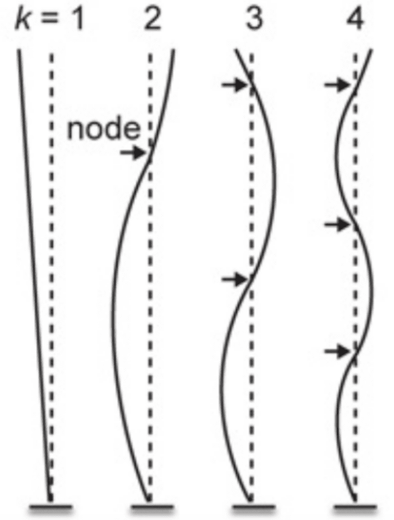
Figure 13: Examples of normal modes of oscillation for a cantilever with a fixed tip, indexed by the integer k, where k = 1 corresponds to the lowest resonant frequency. For a given pattern of vibration corresponding to a normal mode, the value of k can be determined by counting the number of nodes (i.e., points of zero motion, indicated with arrows) (Dakin et al., 2016).
It was found that several features in the tail’s biomechanical design allowed for efficient rattling at very specific frequencies to occur. This is, in part, made possible by the fact that frequencies used during train-rattling are always well-matched to a peak in the resonant response of the peacock’s tail (Figure 14).
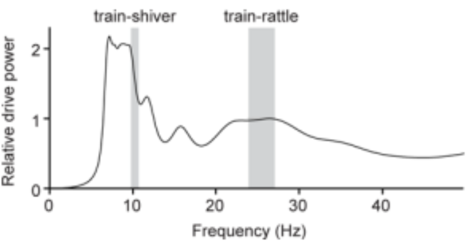
Figure 14: Power spectrum for a peacock’s tail as a function of the vibrational frequency. The tail is shown to have two broad resonant peaks near the average train-shivering and train-rattling frequencies (Dakin et al., 2016).
Indeed, the breadth of the peak in the figure suggests that peacocks can efficiently vibrate their tails to set the train vibrations at a range of frequencies from 22–27 Hz. Conveniently, the minimum of this range corresponds to the broad resonant peak centered at 21.9 Hz found in the figure and overlaps with the vibration frequency of feathers during train-rattling, and the maximum of this range overlaps with the broad k = 3 spectral peak (3 nodes) for the train array at ~27 Hz. There is also another peak centered at 6.9 Hz, which is close to both the average train-shivering frequency and the k = 2 spectral peak for the train array. These findings indicate that the tail should find no issue in setting train vibrations at both the train-rattling and train-shivering frequencies. As a final point, no peak is to be found below ~5 Hz which may explain why we do not see the k = 1 mode excited in the peacock’s train. Ultimately, these agreements in the resonant frequency between the tail and its array of train feathers reduces the effort required to create and sustain vibrations and is thus, considering that their train-rattling can often last for 25 minutes, likely necessary to send the desired signals to the peahen (Dakin et al., 2016).
Finally, to better understand the motion of feathers during shaking and the damping of resonant systems, a spectrogram, which accounts for variation in frequency, was computed. Each kth peak in the function was fitted to a Lorentzian function, a type of bell-shaped curve, which provides a resonant frequency, fk, and a quality factor, Qk. This function can be seen below.
\begin{equation}
Qk=2\pi\frac{energy stored/cycles}{energy dissipated/cycle}=\frac{fk}{\Delta fl,3dB}
\end{equation}
In this function, the value of Δfk,3dB describes the effective width that a resonant peak can have given a significant lowering in the drive power to half of its maximum value at distances of ± Δfk,3dB from the resonant peak at frequency fk. Generally, this means that good resonators with little damping have a Q > 2π with more narrow resonant peaks whereas resonators with great damping have a Q between ½ and and π wider resonant peaks. Because of variations for the length of feathers and for the positions where motion was tracked, the transfer function for each feather was set to a maximum value of 1 (Dakin et al., 2016).
Conclusion
This discussion of various modeling techniques for both avian and fish tails, along with a study of how resonance plays a role in peacock tails, lead to a few different conclusions. All three sections expand on the understanding of the many unique behaviors that tails have adapted throughout evolution. Caudal fins provide a method of propulsion, while avian tails have a role in communication and selection.
It is important to consider how each variable controlling the mechanics of the tail plays into its overall effect on the species. For example, the divergent path of evolution for the stiffness of fish spines and caudal regions can be examined to determine which conformation leads to the most efficiency for propulsive motion. For avian species, the effect of drag during flight must be considered versus how the tail is able to contribute to the steering mechanism. Additionally, the train length, and therefore energy expenditure, must be considered and compared to the resonance capabilities of a peacock.
The study of avian tails is important mainly for the understanding of how beneficial traits can evolve. While fish tails are also interesting for this reason, they also have additional applications within robotics. As discussed, underwater robotic devices are becoming increasingly important. The different characteristics of aquatic tails can be studied to create more efficient underwater robotic propulsive devices. There are also a variety of methods that can be used to determine the efficiency of a modeled robotic tail.
Citations
Dakin, R., McCrossan, O., Hare, J. F., Montgomerie, R., & Amador Kane, S. (2016). Biomechanics of the peacock’s display: How feather structure and resonance influence multimodal signaling. PloS one, 11(4), e0152759. https://doi.org/10.1371/journal.pone.0152759
H. Jane Brockmann, Why are Animals so Honest?, BioScience, Volume 56, Issue 10, October 2006, Pages 849–851, https://doi.org/10.1641/0006-3568(2006)56[849:WAASH]2.0.CO;2
Mitchell, Cody. (2022) Peacocks. World Animal Foundation. https://worldanimalfoundation.org/advocate/farm-animals/params/post/1278208/peacocks
On the aerodynamics of birds’ tails. (1993). Philosophical Transactions of the Royal Society of London. Series B: Biological Sciences, 340(1294), 361–380. https://doi.org/10.1098/rstb.1993.0079
Read, D. A., Hover, F. S., & Triantafyllou, M. S. (2003). Forces on oscillating foils for propulsion and maneuvering. Journal of Fluids and Structures, 17(1), 163-183. https://doi-org.proxy3.library.mcgill.ca/10.1016/S0889-9746(02)00115-9
Root, R. G., & Liew, C. W. (2014). Computational and mathematical modeling of the effects of tailbeat frequency and flexural stiffness in swimming fish. Zoology, 117(1), 81-85. https://doi.org/10.1016/j.zool.2013.11.003
Thomas, A. L. R. (1997, April 1). On The Tails of Birds: What are the aerodynamic functions of birds’ tails, with their incredible diversity of form? BioScience, 47(4), 215– 225. https://doi.org/10.2307/1313075
Thomas, A. L. R. (1997a, April). Correlations between tail morphology and measured flight performance. BioScience. https://doi.org/10.2307/1313075
Triantafyllou, M. S., Triantafyllou, G. S., & Yue, D. K. P. (2000). Hydrodynamics of fishlike swimming. Annual review of fluid mechanics, 32(1), 33-53. https://doi.org/10.1146/annurev.fluid.32.1.33
Usherwood, J. R., Cheney, J. A., Song, J., Windsor, S. P., Stevenson, J. P. J., Dierksheide, U., Nila, A., & Bomphrey, R. J. (2020). High aerodynamic lift from the tail reduces drag in gliding raptors. Journal of Experimental Biology, 223(3). https://doi.org/10.1242/jeb.214809
Wen, L., Wang, T., Wu, G., & Liang, J. (2012). Quantitative thrust efficiency of a self-propulsive robotic fish: Experimental method and hydrodynamic investigation. IEEE/Asme Transactions on Mechatronics, 18(3), 1027-1038. https://doi.org/10.1109/TMECH.2012.2194719