Abstract

Order can be found within the seemingly complex, and perhaps even disordered, processes and shapes that constitute magnetotactic bacteria (MTB). This order can be explained by the concepts of mathematics. First and foremost, the crystalline structures within the magnetosomes of MTB can be modelled mathematically. Magnetite and greigite crystals consist of patterns and symmetry that have been explained by mathematics. It was discovered that these internal crystals consist of different morphologies. Furthermore, the strategical motion of MTB using magnetotaxis can be mathematically interpreted based on varying angles between a magnetic field and concentration gradients. Their Brownian motion also gives rise to more descriptive equations of their motility that depend on the Langevin equations. However, various factors must be considered when applying these equations to model their pathways, including the “run” and “tumble” states of their Brownian motion, as well as the effect of MTB’s chemotaxis. Lastly, models of differential equations can be derived to describe the helical motion of MTB as it relates to their shape and environment. Overall, many studies have been performed on these interesting and unique species of bacteria to understand their structures and motion using the principles of mathematics.

Introduction

In the wise words of Winston Churchill, “Symmetry is often a constituent of beauty”. Beauty and symmetry are abundant in nature in various forms in all organisms. Mathematics serves as a tool to describe this complex, abstract idea through models and measurements. Magnetotactic bacteria (MTB) are composed of unique shapes and structures that contribute to their mathematical beauty. In general, bacteria, including MTB, exist in a variety of different shapes, such as spherical, rod-shaped, or spiral conformations as demonstrated in Figure 1 (Fernanda & Daniel, 2018). This diversity in morphology is advantageous for bacteria. Different shapes provide different advantages in different environments, allowing bacteria to overcome their survival challenges, such as nutrient acquisition, cell division, avoiding predation, as well as optimizing various mechanisms (Young, 2007). The relationship between shape and motility is also very important since motility incurs strong physical and energetic demands on the cell shape. In fact, changing the cell diameter by only 2 μm can increase the amount of energy required for chemotaxis by a factor of 10⁵ (Young, 2007)! While MTBs fall into these general categories of bacteria morphology, their magnetosomes are composed of many intricate shapes that individualize them and separate them from other species of bacteria. These organisms have spent billions of years developing and perfecting their features to arrive at their current morphology, the morphology that mathematically makes sense for them.

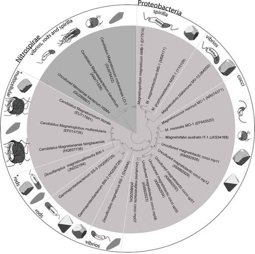
Figure 1: Phylogenetic tree showing the distribution of some cultured and uncultured MTB in Nitrospirae and Proteobacteria phylum of Bacteria domain. White lines separate morphotypes of MTB in Proteobacteria phylum, showing the distribution of spirilla, vibrios, cocci, including ovoid and fava-like cells, rods, and multicellular microorganisms. The shape of magnetosomes found in each morphotypes also displayed next to the cells (Fernanda & Daniel, 2018).

This paper aims to explain various MTB design solutions with the help of mathematics. The first solution covered concerns the sophisticated structure of the magnetosome crystals. Using many mathematical concepts, scientists were able to model and image these crystals to study their construction further. Then, this paper discusses two ways in which MTB motion can be modelled by equations, considering factors like Brownian motion, chemotaxis strategies, shape, and environmental conditions.

Crystallography of Magnetosomes

As was covered in a previous essay, magnetotactic bacteria biomineralize magnetosomes. These are composed of one of two highly structured crystalline compounds: magnetite or greigite. This section will analyse the crystal morphologies and symmetries that have been observed in specific magnetotactic bacterial strains. However, before substantial analysis can be performed, preliminary notions relating to crystallography must be covered to allow a better understanding of magnetosome crystallography and how it benefits the organism’s survival.

Preliminary Notions

Crystals are described as a specific type of mineral that bears flat surfaces and has symmetric relationships with one another (Glazer, 2017). This symmetry is caused by the ordered atomic structures deep within the mineral. Indeed, in nature, there is order and disorder, depending on the patterns observed. In all matter, order introduces many simplifications. It is important to know that there exist two subcategories of order. Long-range translational order occurs when a motif is repeated over lengths longer than the intramolecular scale (Uppsala)[1]. Then, short-range order, most common in all compounds, is the result of constraints of chemical bonds (Uppsala). It follows that there are many degrees of order and, consequently, disorder. Disorder can be defined as the randomness in structure caused by defects, vacancies, and dislocations (Uppsala). It is often caused by randomness in atomic position. Just as order has its subcategories, disorder comes in various ways. The disorder can be structural, oriental, compositional, and vibrational, as illustrated in Figure 2. The most common disorder in amorphous matter is structural, where long-range translational symmetry is not present (Uppsala). Additionally, compositional disorder is recurring in metal alloys, mixtures, and composites (Uppsala). The study of disordered materials is often modelled with random fractals. Fractals are mathematical constructs that exhibit a dilation symmetry (Uppsala). In other words, they look the same on different length scales. Despite allowing considerable simplifications, these random fractals are rarely used to study crystals as these structures have high degrees of order.

For those interested in the concept of random fractals here is a document that describes fractals with greater depth: https://people.bath.ac.uk/maspm/perspectives.pdf

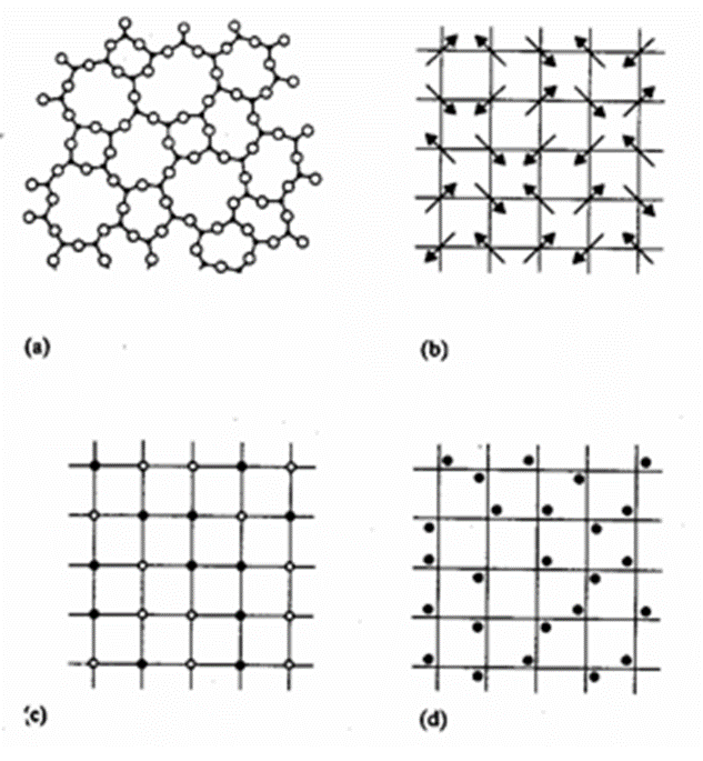
Figure 2: Illustration of various types of disorder; (a) structural, (b) orientational, (c) compositional and (d) vibrational (Uppsala).

Now let us concentrate on the methods that scientists use to study complex crystalline structures, namely X-ray crystallography. During this method, waves, usually in the X-ray range, are propagated onto a crystal sample. These waves will diffract when they interact with the crystalline structure and a pattern will be obtained in the reciprocal space. This imaginary space is created from the direct space in which we find ourselves. Where axes of the direct space are noted by a, b, and c, axes from the reciprocal space are a*, b*, and c* (Glazer, 2017). Additionally, any real axis, a, for example, is perpendicular to reciprocal axes b*, and c*. Figure 3 presents a few points of the reciprocal space constructed from the direct space. It is important to note that units in the reciprocal space are inverse lengths (Lecture 1: Reciporical Space)[2]. On one hand, structures in the reciprocal space are defined in terms of a function F(Q) where Q are the components of wave periodicity obtained from the diffraction pattern (Lecture 1: Reciprocal Space). On the other hand, structures in the real space are density functions r(r), with r as lengths. Both spaces and functions are linked together by the Fourier transform (Lecture 1: Reciprocal Space). The Fourier transform is an equation that allows the deconstruction of a function into a set of waves with different periodicities. The Fourier transform is marked by equation (1) below, while the reverse transform is equation (2) (Lecture 1: Reciprocal Space).

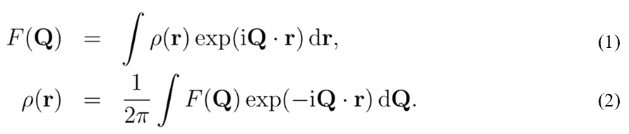
Since X-ray crystallography results in the diffraction pattern of a crystal structure in reciprocal space, the reverse Fourier transform will be more useful for this application.

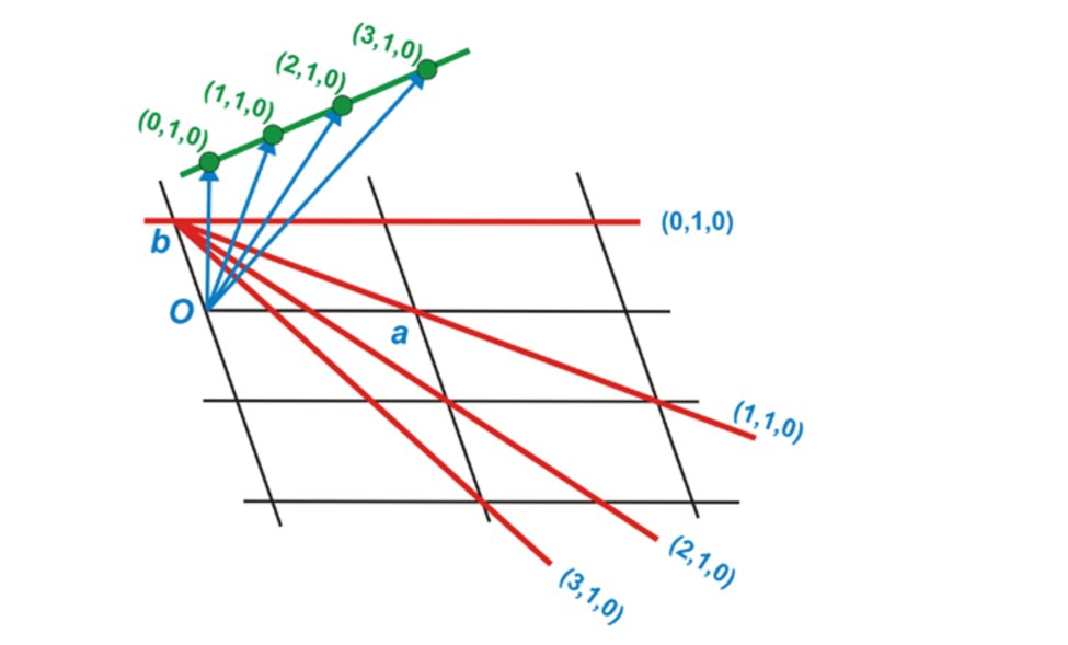
Figure 3: Geometrical construction of some points of a reciprocal lattice (green points) from a direct lattice (black) (Perutz, 1996).

In addition to the Fourier transform, another mathematical operation must be used in the imaging process of a crystal. This operation is the convolution (Lecture 1: Reciprocal Space). Its use is necessary because X-ray crystallography has a limited area on which it sends radiative waves. The idea behind the convolution is that we combine two functions by placing a copy of one function at every point in space defined by the second function (Lecture 1: Reciprocal Space). The idea can be explained by the diagram in Figure 4 below.

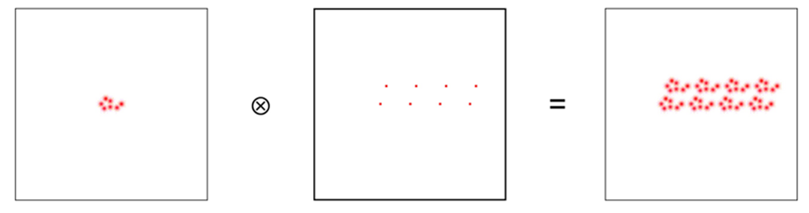
Figure 4: Diagram representing the concept behind the convolution.

The convolution is a useful concept because it allows the deconstruction of a complex structure which in this case would be the crystal. Additionally, the Fourier transform of a convolution is the product of the transforms of both functions (Lecture 1: Reciprocal Space). This simplifies the calculations. While both the Fourier transform and the convolution are universal mathematical concepts, they find a particular use in crystallography because of the crystal nature (Lecture 1: Reciprocal Space). Crystals are minerals with recurring structural unit cells. A unit cell is a region of space that can be repeated by transitional symmetry to fill all the space within a crystal (Glazer, 2017). In other words, the unit cell acts like a motif that would be replicated throughout a mosaic. Figure 5 presents the unit cells for magnetite and greigite, both compounds that occur naturally in magnetotactic bacteria. This particularly pertains to the convolution idea because a crystal can be described as a unit structural cell convoluted with a lattice of points representing the specific tessellation of the crystal.

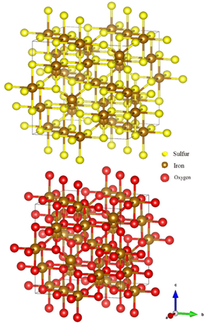
Figure 5: Illustration of the greigite (top), and magnetite (bottom) atomic structures (Nolan, 2018).

Now that both the Fourier transform, and the convolution have been explained, one can see how x-ray crystallography is processed. One needs the Fourier transform of the unit cell, and of the lattice, both of these obtained physically in an experiment (Lecture 1: Reciprocal Space). Then, both are multiplied to get the transform of the crystal. Finally, the reverse Fourier transform can be taken, and the crystal structure in real space is the result.

The next preliminary notion that needs to be covered is Miller indices. These indices provide a labelling system for crystal faces based on the real axes a, b, and c (Glazer, 2017). These axes must not always be perpendicular to one another; the angles between them can vary (Glazer, 2017). The surfaces will be labelled with values h, k, and l with the following notation (h, k, l) (Glazer, 2017). these values represent the points where the plane cuts through the axes. In Figure 6, the conventions for the axes and their surfaces are illustrated (Glazer, 2017).

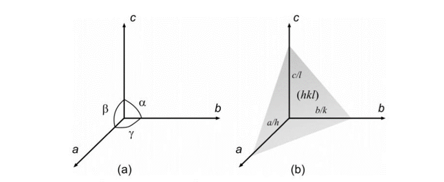
Figure 6: a) convention for the choice of axes. b) definition of a plane (Glazer, 2017).

An additional convention occurs when the h, k, and l values are negative. Instead of adding a minus sign in front, a bar is added on top of the value (Glazer, 2017). Below is presented the nomenclature for the faces of a cube and an octahedron as an example (Figure 7) (Glazer, 2017). Finally, axes can be added for some complex crystal structures like quartz (Glazer, 2017).

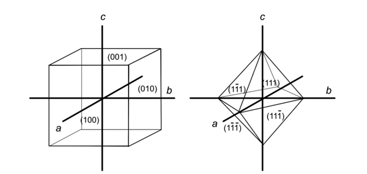
Figure 7: Miller indices for the front faces of a cube and an octahedron (Glazer, 2017).

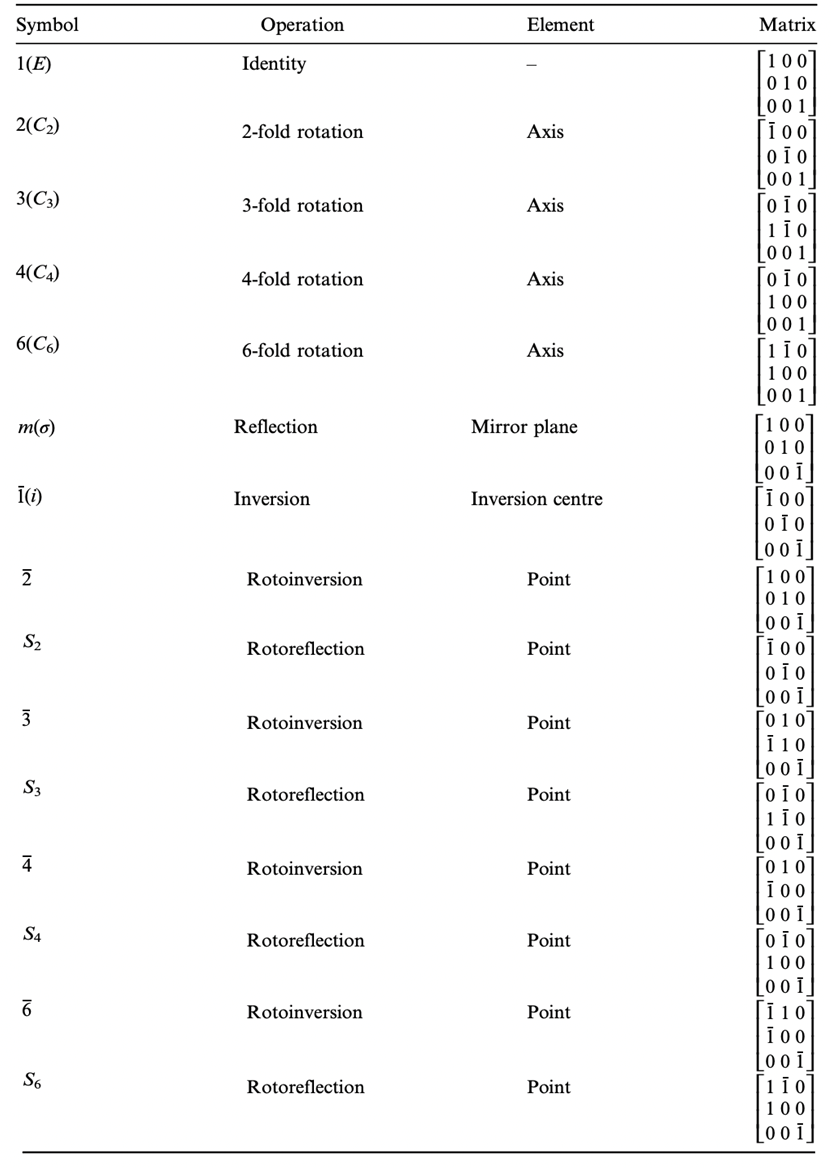
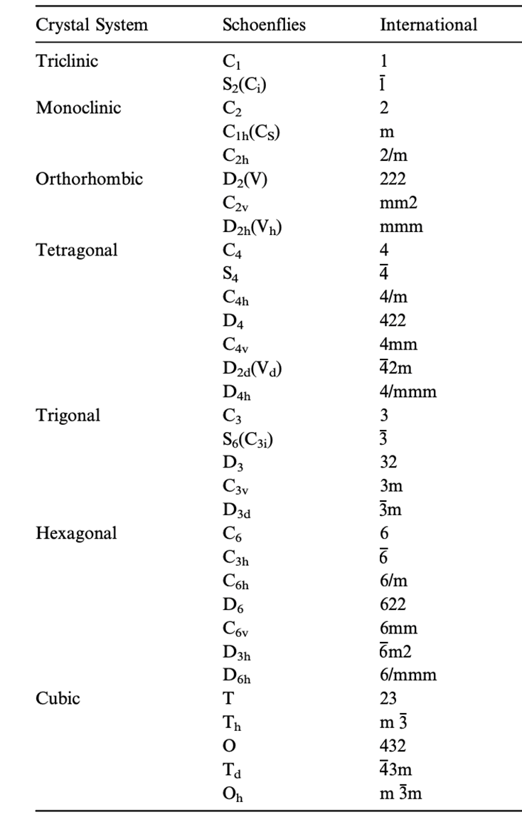
Not only are crystals highly ordered in structure, but they are also ordered in categories by scientists. So far there have been seven crystal systems based on the primitive Bravais lattices proposed, and each contains various numbers of subgroups for a total of 32 crystal subgroups (Glazer, 2017; Rogers, 1926). These different classifications are based on combinations of symmetry operations. These operations are movements with which one can obtain every surface of the general form of the crystal from an arbitrarily selected surface (Glazer, 2017). The first operation is the identity operation. This operation applied on a surface results in the same surface. The second operation is the rotation of a surface about an axis. The rest of the symmetry operations are the reflection or inversion in a plane, the rotary reflection, and the rotary inversion. These operations can be represented by either a symbol or a matrix, both of which are present in the table I in the appendix. Reflections or inversions are straightforward. The reflection occurs at every point in an object as if it were through a mirror (Glazer, 2017). The inversion occurs about a centre of symmetry and can be thought of as rotating an object by 180 degrees and reflecting it across the plane of this angle. An inversion is illustrated in Figure 8 (Glazer, 2017). Lastly, the rotary inversions and rotary reflections are combinations of rotations and inversions (Glazer, 2017).

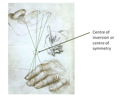
Figure 8: Drawing of the hands of Erasmus of Rotterdam by Holbein (1523). Lines are added to identify the inversion relationship (Glazer, 2017).

Table II in the Appendix presents the classifications of the 32 crystal subgroups and the combinations of operations associated with them (Glazer, 2017). The following section will focus on crystals in the cubic system, more specifically in the hexoctahedral subgroup O_h (Glazer, 2017).

Magnetosome Crystals

Magnetosome crystals, namely magnetite and greigite, have crystal habits belonging to the cubic hexoctahedral group (O_h) (Pósfai et al., 2013). This group is characterized by a combination of 48 symmetry operations which renders its analysis very complex (Glazer, 2017). Although all magnetotactic bacteria contain either magnetite or greigite, the precise shape of the crystals is strain-specific. The small differences notwithstanding, magnetosomal crystals are still classified under the same geometric crystal groups.

In magnetite-producing bacteria, there have been three idealized crystal habits observed based on the combination of low index surfaces (100) (110), (111) (Pósfai et al., 2013). These habits are the cuboctahedral, elongated octahedral, and elongated-anisotropic habits. Figure 9 illustrates the crystal habits of magnetosome crystals. The Miller indices in the following paragraphs can be quite confusing so following along with the figures included is strongly recommended.

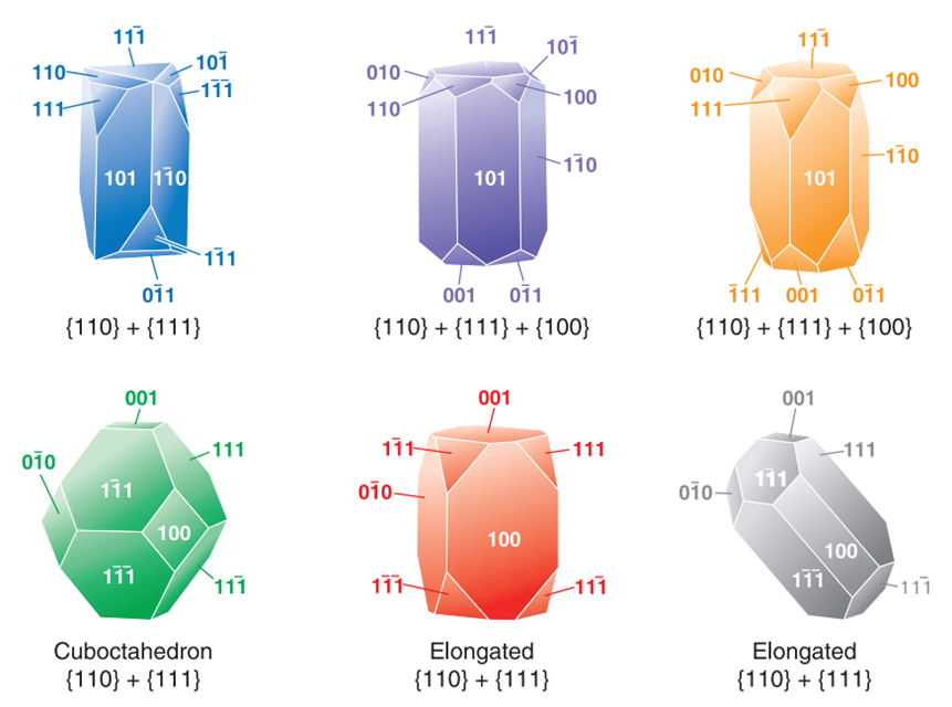
Figure 9: Idealized habits of magnetosome crystals (Frankel & Bazylinski, 2004).

The first habit is often observed in the Alphaproteobacteria phylum under the Magnetospirillium genus. Cuboctahedral morphologies usually consist of six equivalent faces of the (100) form combined with eight equivalent faces of the form (111) (Pósfai et al., 2013). This habit preserves the symmetry associated with the cubic crystal system, making it the closest habit to the equilibrium growth form of the magnetite (Pósfai et al., 2013). In other words, magnetotactic bacteria that synthesize magnetite crystals in a cuboctahedral shape will benefit from the high thermostability of the crystal (Pósfai et al., 2013). Thus, less energy is required from the bacteria to accomplish biomineralization. This can be seen as an adaptation to optimize energy expenditure in the cell (Pósfai et al., 2013). Very similar to the cuboctahedra, magnetospirillium bacteria will also synthesize magnetosomes in octahedral shapes. This morphology is composed of eight (111) faces as demonstrated in Figure 10 (Pósfai et al., 2013). It benefits the bacteria in the same way as the cuboctahedra (Pósfai et al., 2013). Figure 10 also provides the image of the Fourier transform of a cuboctahedral magnetosome in the inset of C. The set of points in this image permitted scientists to infer the specific shape of the crystal (Pósfai et al., 2013).

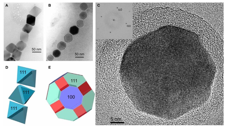
Figure 10: A) Transmission electron microscope image of a partial chain of regular octahedra. B) Transmission electron microscope image of a partial chain of cuboctahedral magnetosomes. C) High resolution TEM image of a cuboctahedral magnetosome, witht the Fourier transform inserted in the upper left corner. D) Schematic model for the octahedra in A). E) schematic model for the crystal shown in C) [Adapted from Pósfai et al., 2013].

The cuboctahedral and, by extension, octahedral habits are the only equidimensional habits observed in magnetotactic bacterial strains. All other habits are elongated. One of the most common among these habits is the elongated octahedral depicted in Figure 11 (Pósfai et al., 2013). This habit is an octahedral with enhanced growth in the direction parallel to the (111) planes.

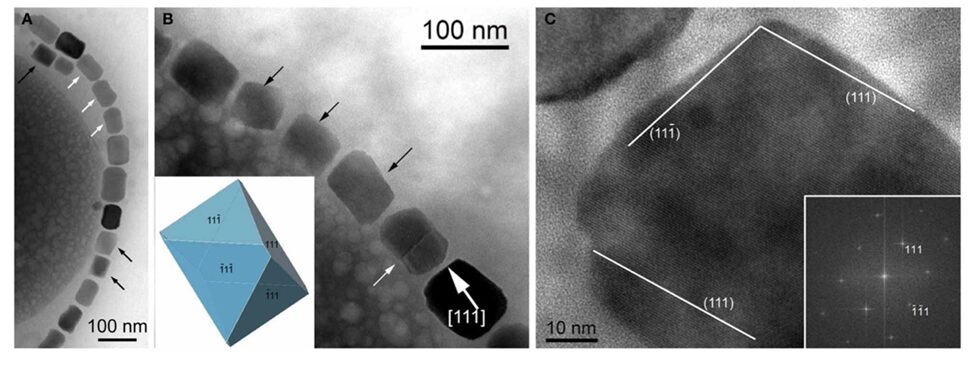
Figure 11: A) Transmission electron microscope image of a chain with highly elongated magnetosomes. Black arrows mark magnetosome with pronounced octahedral facets. B) TEM image of a partial chain of cuboctahedral magnetosomes. The circled white arrow shows elongation along the (111) axis. C) High resolution TEM image of the magnetosome in the lower right of B) the Fourier transform is present in the lower right corner.

Additionally, magnetotactic bacteria can form elongated cuboctahedral magnetosomes (Pósfai et al., 2013). This last morphology introduces faces of the (110) form. Indeed, it is constructed from six (110) faces, two larger and six smaller (111) with six (100) faces (Figure12) (Pósfai et al., 2013). Again, this morphology is elongated in the (111) direction. Such elongations create forms with no centre of symmetry. This means that the crystal is different from its ideal equilibrium shape (Pósfai et al., 2013). While this might require the bacteria to expend more energy in the magnetosome formation, the elongation aligns with the easy magnetization axis of the magnetotactic bacteria. Thus, maximizing the magnetic moment of the crystal (Pósfai et al., 2013).

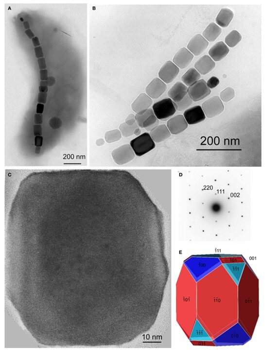
Figure 12: A) TEM image of a cell containing a chain of elongated magnetosomes. B) TEM image of two double chains of elongated magnetosomes. C) High resolution TEM image of a magnetosome. D) the diffraction pattern of the elongated magnetosome. E) Morphological model of an elongated cuboctahedral magnetosome. The elongated direction is (111) [Adapted from Pósfai et al., 2013].

The last crystal habit is observed in Deltaproteobacteria, more specifically in the Nitrospirae phylum. This crystal habit is called the elongated-anisotropic habit, and it is usually characterized by a bullet-shaped crystal with a flat top (Pósfai et al., 2013). These habits can take many configurations such as presented in Figure 13. Some of these elongated anisotropic crystals have distinctive projected images with two isosceles triangles sharing a base (seen in Figure 12C) (Pósfai et al., 2013). The images obtained by transmission electron microscopy (TEM) reveal little information on the actual geometry of the crystal. That is why Figure 14 modelled the crystal shapes based on the Fourier transform (Pósfai et al., 2013). In this Figure, one can see that higher indexes are necessary to represent the surfaces. Similar to the other elongated crystals, the elongation direction is usually parallel to (111), although bending can occur, and sections may have different elongation directions. This was specifically selected by evolution for the stronger magnetic moment it provides the magnetosome (Pósfai et al., 2013).

Referring to the composition of greigite magnetosomes, one can see that sulfur atoms occupy the place that oxygen atoms have in magnetite. Although magnetite and greigite have very similar structural units, the different atoms will have a great impact on the overall morphology of the crystal. Sulfur has different chemical properties from oxygen. For example, the element’s size, electronegativity, and covalence are different (Roldan, Santos-Carballal, & de Leeuw, 2013). This will have repercussions on the distance and the strength of the bonds between atoms, thus, altering the short-range order of the crystal. Although these changes are minor in the order of the structural cell unit, they are amplified in the overall crystal morphology because of the long-range order. The translational symmetry present in mineral crystal is as important as the motif behind it.

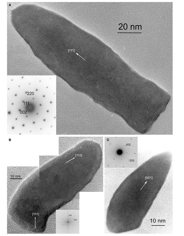
Figure 13: Images of magnetite magnetosomes with highly anisotropic, elongated, pointed habits. A) A magnetosome elongated to (111), with the diffraction pattern in the lower left. B) a composite image of a curved magnetosome in the (110) direction with its Fourier transform in the lower right. C) A magnetosome isosceles triangle bases elongated in the (001) direction [Adapted from Pósfai et al., 2013].

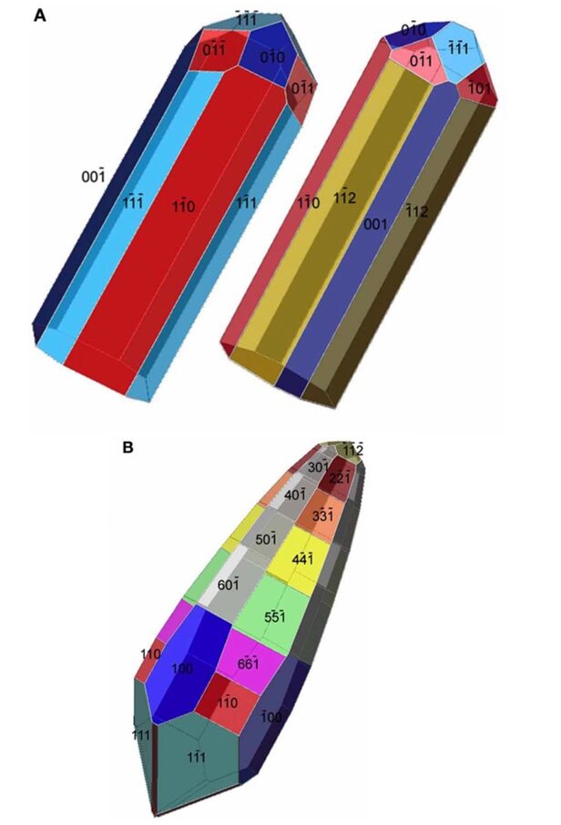
Figure 14: Tentative models for the elongated magnetosomes in Figure 13. A) two possible morphologies for the magnetosome in A) and B) of Figure 13. B) An approximate model for the morphology of the magnetosome in Figure 13 C) [Adapted from Pósfai et al., 2013].

While it would be interesting to dive deeper and perform detailed analyses of the differences between biological magnetite and greigite crystal habits, current scientific knowledge on greigite magnetosomes is very limited. In fact, only one strain of greigite-producing bacteria is able to be cultured (Pósfai et al., 2013). However, these bacteria have been observed in collected samples, and it is believed that the precise greigite morphologies are also strains and species-specific (Pósfai et al., 2013). Usually, greigite crystals contain planar defects among their layers which results in fairly irregular crystal shapes (Pósfai et al., 2013). This can be observed precisely in Figure 15 C). Through the irregularities, there have also been numerous accounts of slight elongation parallel to the (100) axis. Just like magnetite magnetosomes, this is believed to optimise the magnetization of the crystal, a crucial aspect of the cell’s navigation system (Pósfai et al., 2013). In essence, the understanding of the shapes and geometrical principles that are present in magnetotactic bacteria’s magnetosomes reveals plausible reasons as to why these organelles have evolved to the way they are now.  

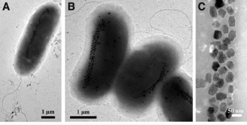
Figure 15: Transmission electron microscope (TEM) images of uncultured, large, greigite- and/or magnetite-producing, rod-shaped bacteria. A) and B) TEM images of greigite producing magnetotactic bacteria. C) High-magnification TEM image of greigite crystals from the cells shown in B) (Lefèvre et al., 2011).

Predicting the Magnetotactic Advantage: A Statistical Mechanics Approach

The ability of MTB to swim along concentration gradients to optimally situate where desired substrates are located and where repellants are avoided is crucial. This is especially important for following the oxic-anoxic interface (OATZ), which is a specific layer near the surface of chemically stratified waters where their specific oxygen concentration levels can be found (Figure 16). Since the OATZ moves rapidly near the surface of the water, MTB must have rapid chemotactic strategies that allow them to follow the OATZ (Frankel, Williams, & Bazylinski, 2007). MTB that live near the Southern or Northern hemispheres benefit from the presence of a vertical component to the Earth’s magnetic field. This allows them to swim along the direction of the oxygen gradient, and away from high oxygen concentrations near the atmosphere (see Figure 16). However, the advantage of magnetic field alignment is not obvious for MTB located near the equator, where magnetic field lines lack a significant vertical component. It becomes relevant to address the effects of increasing angles between magnetic field lines and the gradient of a substrate of importance like oxygen, to predict the magnetotactic advantage and explore the different strategies possibly adopted by MTB to follow gradients optimally. An appropriate model developed by Codutti et al. that considers known bacterial chemotaxis strategies, such as the run and tumble and run and reverse (typical in MTB), as well as the statistical physics of Brownian motion affecting MTB, is described below. This mathematical model does fully capture MTB motion, but it turns out that although varying angles between a magnetic field and concentration gradients affect aerotactic response, relatively low angles result in faster aerotactic responses in the presence of a magnetic field, and angles close to the 90° result in slower but unhindered aerotaxis, in line with the existence of MTB close to the Earth’s equator (Codutti et al., 2019).

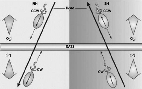
Figure 16: Downward movement of MTB situated in the Northern (right) or Southern (left) hemispheres, along magnetic field lines with a strong vertical component. Oxygen concentrations increase above the OATZ. The mention of reduced sulfur compounds, indicated to increase in concentration below the OATZ, hints at another taxis whereby reduced sulfur compounds are detected to aid in triggering a reversal in movement, allowing to remain at the OATZ (Frankel, Williams, & Bazylinski, 2007).

Modeling MTB as an Active Brownian Particle

The concept of Brownian motion is important to describe the effects of thermal noise on a particle of interest. Brownian motion describes how a particle immersed in a fluid moves because of its collisions with surrounding particles, also referred to as thermal noise. The example provided in Figure 17 shows a larger particle M surrounded by smaller fluid particles that collide with it frequently.

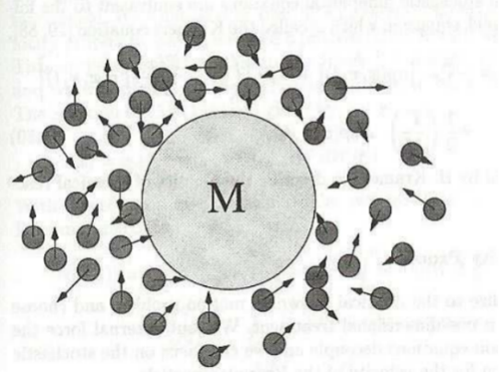
Figure 17: Brownian particle M surrounded by smaller fluid particles which collide frequently with the Brownian particle (“Brownian Motion: Langevin Equation”).

Because of the large number of collisions around the particle of interest (this can go up to 10¹⁴ collisions between gas molecules, for instance), no cumulative force is experienced most times. Occasionally, significant net forces on the particle cause it to “jump” in a random direction (referred to as a random walk). This is the basis of Brownian motion, and it is useful to treat bacteria like MTB as Brownian particles in water. MTB are considered active particles, as they are self-propulsive and exhibit a rotational bias due to chemotaxis. The forces relevant to Brownian motion are included in the Langevin equation:

m (d(v(t) ) ⃗)/dt= -γ(v(t) ) ⃗+(ε(t) ) ⃗+(F_{ext} ) ⃗

In this form of Newton’s second law of motion, -γv(t) represents the drag force from the fluid around the Brownian particle (proportional to its velocity and a drag coefficient γ), ε(t) is a random force generated by thermal noise around the Brownian particle, and F_ext is any external force (e.g. gravity, external magnetic field).

In a recent model of MTB motion under concentration gradients (of any substance) and magnetic fields (developed by Codutti et al.), active Brownian motion is comprised of two states. The first is the “run” state, which occurs when MTB particles move at an uninterrupted pace, and the second is the “change in direction” state, characterized by a sudden stop in self-propulsion and subsequent reorientation. These states are accounted for in two rewritten forms of the Langevin equation, which describe the translational and rotational motion of an active Brownian point particle. The translational motion of a particle MTB at position r is implicitly described by:

γ_t  (dr ⃗)/dt= γ_t σve ⃗+(F_{ext} ) ⃗+√(2k_B Tγ_t )* (ε_t ) ⃗

Here, γ_t is a translational drag coefficient, v is the point particle’s self-propulsion speed, e provides the direction of movement, K_B is the Boltzmann constant, and T is the temperature at the location of the particle. ε_t is a noise vector, analogous to ε(t) in the original Langevin equation, in the translational degree of freedom. Also, σ is a scalar quantity of importance, as it determines the state of the MTB as an active Brownian particle: σ takes the values of -1 or 1 for runs (anti-parallel or parallel to the concentration gradient) and 0 for tumbles.

γ_r  (de ⃗)/dt=((T_{ext} ) ⃗+√(2k_B Tγ_r )*(ε_r ) ⃗ )  ×e ⃗  

The expression on the right-hand side denotes the cumulative contributions of rotational forces (an external torque T_ext and a random torque √(2K_BTγ_r) ∗ ε_r arising from thermal noise) on the direction vector e, which is proportional to the change in e over time. This time, γ_r is a rotational drag coefficient. Now, changes in direction caused by a tumble and transition from the tumble state to the run state require a rapid reorientation, where the noise strength at the point of the Brownian particle is greater than surrounding thermal noise. This is modeled by defining a “tumble temperature” T_tumble at a localized point of the Brownian particle that must be higher than the surrounding temperature to induce rapid reorientations during a tumble. T_tumble is not the ambient temperature and serves only to simulate the distribution of orientations over time during a tumble (i.e. tumbles are “considered” to be thermal agitations that affect the particle’s motion). This is used as a variable temperature parameter in the Langevin equations to simulate tumbles in a computer program. For the simulation, a T_tumble = 4.2 ∗ 10⁴ K is used (in accordance with past experiments on E. coli), which is significantly greater than ambient temperature.

Considering Chemotaxis

Although they are simulated using the Langevin equations, tumbling events are driven by chemotaxis, whereby a change in direction provides an opportunity to move towards optimal concentrations of a particular substance. Taken again from the well-studied E.coli, the average tumble time (τ_tumble = 0.1 s) is much smaller than the average run time (τ_run ≅ 1 s). Tumble time is considered to remain constant, but τ_run depends on the movement of MTB along the concentration gradient, where

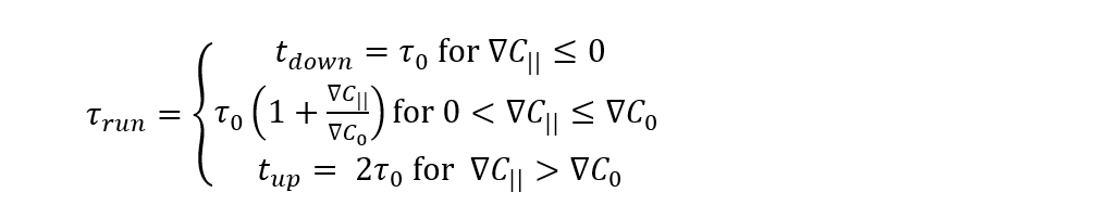
Here, τ₀ is the average run time in the absence of a concentration gradient, ∇C_|| is the component of the concentration gradient along the direction of motion, and ∇C₀ is a threshold gradient that changes MTB. This only provides τ_run when considering a concentration gradient for an attractant (i.e. a desired substrate, which may become a repellant up to a certain threshold). So, when ∇C_|| ≤ 0, MTB are moving down the gradient, which is not beneficial for following an attractant. This is the reason for which t_down < t_up. When ∇C_|| is confined below ∇C₀, the run time τ₀(1 + ∇C_||/∇C₀) increases as ∇C_|| approaches the threshold above which the highest run time t_up is reached (high attractant concentrations). The expression for τ_run under the concentration gradient of a repellant is analogous to that with an attractant, and contributions from all substrates may be considered.

The run and reverse model of motion in MTB is analogous to the run and tumble movement. However, run-and-reverse is more relevant to MTB as an instantaneous direction reversal is more effective for following a concentration gradient under an imposed magnetic field. One interesting fact is that orientational noise is only thermal in the run and reverse motion. This is an advantage for MTB compared to non-magnetic bacteria like E. coli, which change direction through the additional energy-consuming step of orienting flagella before reorienting them along the axis of motion.

Movement Strategy: Influence of Magnetic Field

In practice, MTB benefits from both strategies (reversals and tumbling), so it becomes important to understand which conditions lead to favoring one solution over another. One such condition includes the influence of a magnetic field on the motion of run and tumble. An external magnetic field imparts a torque

T ⃗_{ext}=M ⃗×B ⃗,

where M is the magnetosome chain’s magnetic moment and B is the magnetic field. However, tumbles disturb magnetic alignment and are followed by a relaxation time required for realignment to occur (see Figure 18 a)). This relaxation time is given by τ = (||B|| ||M||γ_r^-1)^-1

(this logically increases with higher rotational drag, and with lower magnetic field and magnetic moment strengths). Subsequent tumbles may perturb the process of realignment, i.e. when τ_run < τ, MTB do not have enough time to align with B. Again, to include this in the model for MTB motion, the Langevin function for magnetism is considered. In the absence of any form of mechanical noise, the energy of alignment of a magnetic dipole with a magnetic field is given by

E= -M ⃗∙B ⃗=-‖B ⃗ ‖‖M ⃗ ‖  cos⁡θ  

Where θ is the angle of magnetic alignment. However, the natural presence of thermal noise causes fluctuations in magnetic alignment, which gives rise to a probabilistic distribution (arising from Boltzmann statistics) of alignment angles for a given alignment energy. This factor is considered in the Langevin function for magnetism, which provides the mean alignment angle

〈cos{⁡θ_{e ⃗,B ⃗ }}  〉  =coth⁡{(‖B ⃗ ‖‖M ⃗ ‖/(k_B T_{eff} ))-} (‖B ⃗ ‖‖M ⃗ ‖/(k_B T_{eff} ))^{-1}

Here, the effective temperature T_eff is a new constant (not the same as T_tumble, which is only used to model MTB under no magnetic field) that considers the competition between the mean run time before a tumble and the relaxation time for realignment. Again, T_eff is not the ambient temperature, but rather a way to simultaneously model the weighted effect of tumbling and relaxation as if they were thermal effects. The value of T_eff is an interpolation between the noise strength of tumbling and the actual surrounding temperature and is obtained by curve fitting of the Langevin function on data points plotted from different simulated runs (Figure 18 b)). As seen in Figure 18 d), the average alignment angle is greater with T_eff than at ambient temperature, which owes to the effect of tumbling. Also, the dependency of the run time on the effective temperature is shown in Figure 18 c).

The Full Picture

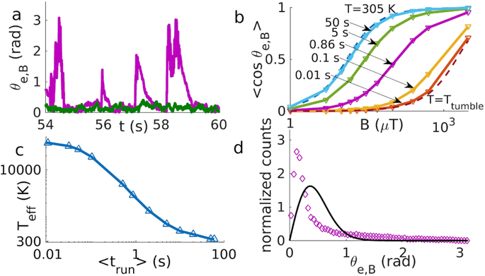
Figure 18: a) The alignment angle against time for run and reverse (purple) and run and tumble (green) with run time of 0.86s and magnetic field 500 µT. b) Langevin plots, each corresponding to different run times. Theoretical lines are dotted and bound the interpolation range over which Teff is estimated (corresponding to purple fit curve). c) Teff dependency on mean run time (fitted curve). d) Alignment angle distribution for the run and tumble strategy at Teff (black curve) and from data points at 305K (data points), where mean run time is 0.86s and magnetic field strength is 500 µT (Codutti et al., 2019).

The mathematical relationships that have been revealed so far allow testing of different situations where MTB will have to respond using the different strategies discussed (i.e. chemotactic run and tumble, and run and reverse). Figure 19 shows the mean effective velocity of MTB, which is the component of velocity along the concentration gradient direction, against the angle of inclination between the magnetic field and the concentration gradient. Different conditions are in the figure to show the effect of magnetic fields, as well as the adoption of each separate motility strategy. ❬v_taxis❭ is obtained by taking the projection of the velocity of MTB along the direction of the concentration gradient. Because of thermal noise and other forms of noise (e.g. tumbling), the orientation of MTB relative to the magnetic field is given by the Langevin function. So, to obtain ❬v_taxis❭, it is sufficient to project the velocity of MTB along the magnetic field, which will be projected anew along the direction of a concentration gradient. The relationship for this is given by

v_{taxis}≅v cos⁡{{(θ}_{B,∇C})} (coth⁡{(‖B ⃗ ‖‖M ⃗ ‖/(k_B T_{eff} ))-} (‖B ⃗ ‖‖M ⃗ ‖/(k_B T_{eff} ))^{-1} )

Here, v is the velocity of MTB along the direction of its motion. This relation can describe the velocity for tumble taxis, but it would need modification in the case of reverse taxis velocity, which is given by

v_{reverse taxis}≅v {|cos}⁡{{(θ_{B,∇C}  )}|} (coth⁡{(‖B ⃗ ‖‖M ⃗ ‖/(k_B T_{eff} )})- (‖B ⃗ ‖‖M ⃗ ‖/(k_B T_{eff} ))^{-1} )  (t_{up}-t_{down})/(t_{up}+t_{down}+ {2t}_{pause} )

Here, the absolute value of cos(θ_{B, ∇C}) is taken, as reverse taxis involves motion both parallel and antiparallel to the gradient, which is not an indicator of disadvantageous taxis (denoted by negative taxis velocities). Instead, the expression (t_up – t_down)/(t_up + t_down + 2t_pause) is used to provide a normalized direction of motion, depending on the difference between the time t_up spent swimming up the gradient (advantageous contribution) and the time t_down spent swimming down the gradient (disadvantageous contribution). These are the equations that allow to reproduce Figure X, which shows which strategies are preferrable under different orientations between the magnetic field and the concentration gradient (θ_{B, ∇C}). Importantly, tumble motion (dotted and pink) is associated with higher taxis velocities for small θ_{B, ∇C} (below 90°), but reverse motion can be employed to obtain efficient taxis velocities for  θ_{B, ∇C} exceeding 90°, which would be otherwise disadvantageous with tumbling. This illustrates the complementary nature of these two strategies, which have been observed in MTB. However, at θ_{B, ∇C} = 90°, both tumbling and reverse strategies (pink lines) provide no advantage under a magnetic field of 50 µT and even the absence of a magnetic field (green lines) is associated with a positive taxis velocity at θ_{B, ∇C} = 90°. However, in simulated experiments performed by Codutti et al., the formation of aerotactic bands by MTB still occurs at θ_{B, ∇C} = 90°, which is in line with the fact that MTB are found near the equator of the Earth.

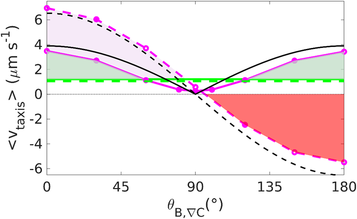
Figure 19: Taxis velocity dependency on relative orientation between magnetic filed and concentration gradient. Dotted lines are for run and tumble, and continuous represent run and reverse motion. Black lines are theoretical. Pink lines are obtained at 50 µT. Green lines are obtained at 0 µT (Codutti et al., 2019).

Additionally, a significant advantage of magnetic field alignment is the significant reduction in rotational diffusion by thermal noise. This is especially important in MTB, as they have been observed to have much longer runs than E.coli (about 2s), which might hinder their ability to navigate optimally along concentration gradients in the absence of magnetic fields as illustrated in Figure 20 (increased taxis). It is remarkable that the curves of taxis velocities plateau for increasing upward gradient run times, which shows the significant advantage of magnetic field alignment.

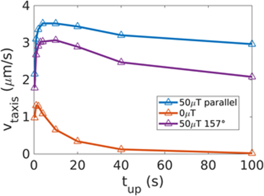
Figure 20: Taxis velocities plotted as a function of time spent swimming up a concentration gradient (Codutti et al., 2019). Legend assigns color to a corresponding magnetic field under which simulated particle swims.

Evident advantages mentioned above stem from magnetic field alignment and the adoption of different motility under varying conditions. Also, it has been shown through simulations that aerotactic band formation is faster under low θ_{B, ∇C}. However, even though tumbling and reverse motion have been observed in MTB, it remains unknown how these organisms apply these strategies under different conditions.

Conclusion

Ultimately, magnetotactic bacteria synthesize their magnetosomes with different morphologies to optimise magnetotaxis and thermostability. The morphologies, which rely on numerous mathematical concepts, can be slightly different from species to species. Although the precise cause for these changes remains debated, one could conclude that the variations are slight adaptations to each species’ microenvironments. Alternatively, discrepancies could have risen as small benign mutations in the bacteria’s genome. Then again, one similarity between magnetosomes regardless of their chemical composition is their slight elongation in one direction. This enhances the magnetization of the organelle which in turn, increases the bacteria’s navigating skills. Moreover, the strategies that magnetotactic bacteria use to navigate in their environment are constrained by key factors such as concentration gradients of different attractant or repellant substances, as well as magnetic field alignment and Brownian motion due to thermal noise. To follow concentration gradients optimally, magnetotactic bacteria are equipped with run and tumble and run and reverse movement patterns, which are advantageous for complementary ranges of angles of alignment between the magnetic field and a concentration gradient of interest. This provides a significant advantage for MTB, which can exhibit both run and tumble and reverse behaviours. These design solutions also owe to the fact that magnetotactic bacteria have been observed near the equator, where magnetic field lines are orthogonal to oxygen concentration gradients. While mathematics may not be used by the organisms themselves, they can be very useful tools for scientists to gain further knowledge on natural mechanisms and design solutions to possibly replicate these solutions in particular applications.

References

Batchelor, G. K. (1967). An Introduction to Fluid Dynamics. Cambridge: Cambridge University Press.

Brownian Motion: Langevin Equation. In. http://web.phys.ntnu.no/~ingves/Teaching/TFY4275/Downloads/kap6.pdf

Cui, Z., Kong, D., Pan, Y., & Zhang, K. (2012). On the swimming motion of spheroidal magnetotactic bacteria. Fluid Dynamics Research, 44(5), 055508. https://doi.org/10.1088/0169-5983/44/5/055508

Codutti, A., Bente, K., Faivre, D., & Klumpp, S. (2019). Chemotaxis in external fields: Simulations for active magnetic biological matter. PLoS Comput Biol, 15(12), e1007548. https://doi.org/10.1371/journal.pcbi.1007548

Fernanda, A., & Daniel, A.-A. (2018). Biology and Physics of Magnetotactic Bacteria. In B. Miroslav, S. Mona, & E. Abdelaziz (Eds.), Microorganisms (pp. Ch. 1). IntechOpen. https://doi.org/10.5772/intechopen.79965

Frankel, R., & Bazylinski, D. (2004). Magnetosome mysteries. Despite reasonable progress elucidating magnetotactic microorganisms, many questions remain. Physics, 70, 176-183.

Frankel, R., Williams, T., & Bazylinski, D. (2007). Magnetoreception and magnetosomes in bacteria: Magnetoaerotaxis. 2-24.

Glazer, A. M. (2017). A journey into reciprocal space: a crystallographer’s perspective. Morgan & Claypool Publishers.

Koiller, J., Ehlers, K., and Montgomery, R. (1996). Problems and progress in microswimming. J. Nonlin. Sci. 6, 507–541. doi: 10.1007/BF02434055

Kong, D., Cui, Z., Pan, Y., and Zhang, K. (2012). On the Papkovich-Neuber formulation for Stokes flows driven by a translating/rotating prolate spheroid at arbitrary angles. Int. J. Pure Appl. Math. 75, 455–483.

Lecture 1: Reciprocal Space.  http://goodwin.chem.ox.ac.uk/goodwin/TEACHING_files/l1_handout.pdf

Lefèvre, C., Menguy, N., Abreu, F., Lins, U., Pósfai, M., Prozorov, T., Pignol, D., Frankel, R., & Bazylinski, D. (2011). A Cultured Greigite-Producing Magnetotactic Bacterium in a Novel Group of Sulfate-Reducing Bacteria. Science (New York, N.Y.), 334, 1720-1723. https://doi.org/10.1126/science.1212596

Papkovich, P. F. (1932). The representation of the general integral of the fundamental equations of elasticity theory in terms of harmonic functions (in Russian). Izr. Akad. Nauk. SSSR Ser. Mat. 10, 1425–1435.

Perutz, M. (1996). Direct and Reciprocal Lattices [Online Texbook]. https://www.xtal.iqfr.csic.es/Cristalografia/parte_04-en.html

Pósfai, M., Lefèvre, C., Trubitsyn, D., Bazylinski, D., & Frankel, R. (2013). Phylogenetic significance of composition and crystal morphology of magnetosome minerals [Review]. Frontiers in Microbiology, 4. https://doi.org/10.3389/fmicb.2013.00344

Rogers, A. F. (1926). A Mathematical Study of Crystal Symmetry. Proceedings of the American Academy of Arts and Sciences, 61(7), 161-203. https://doi.org/10.2307/20026154

Roldan, A., Santos-Carballal, D., & de Leeuw, N. H. (2013). A comparative DFT study of the mechanical and electronic properties of greigite Fe3S4 and magnetite Fe3O4. J Chem Phys, 138(20), 204712. https://doi.org/10.1063/1.4807614

Uppsala. Order and Disorder. In (pp. 8). Sweden. https://www.teknik.uu.se/digitalAssets/386/c_386360-l_3-k_disorder_intro.pdf

Young, K. D. (2007). Bacterial morphology: why have different shapes? Curr Opin Microbiol, 10(6), 596-600. https://doi.org/10.1016/j.mib.2007.09.009

Appendix

Table I: Crystallographic Symmetry Operations

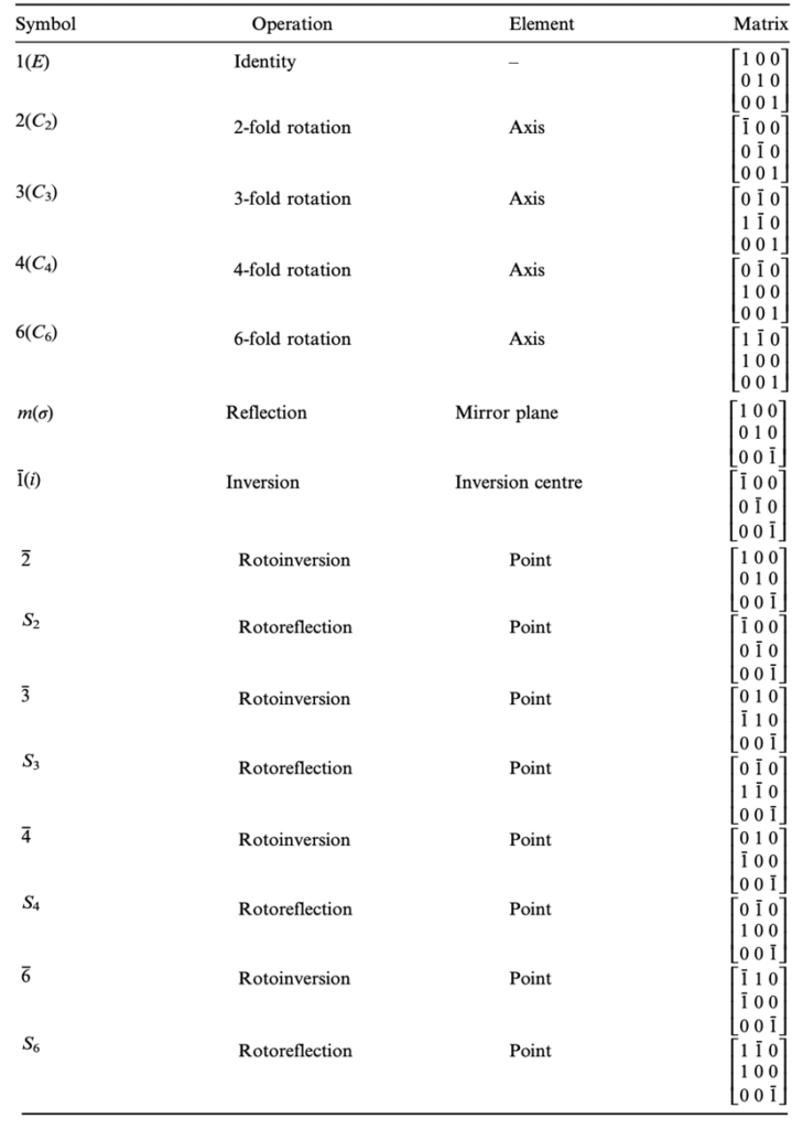
Adapted from (Glazer, 2017)

Table II: The Seven Crystal Systems and 32 Geometric Crystal Subgroups

Schoenflies and International are the two accepted notations.

Adapted from (Glazer, 2017)

Here is additional content on the shape dependency of magnetotactic bacterial motion (Appendix situated below for later reference)

Using Mathematical Models to Describe Swimming Patterns

This section presents another approach to modelling the magnetotactic bacteria’s helical motion. This motion, a design solution used by most bacteria, varies under many factors. Just like for any model, assumptions must be made to simplify equations.

The first assumption made concerns the shape of the magnetotactic bacteria. The most prominent shape in magnetotactic bacteria species is the rod. Rod-shaped magnetotactic bacteria can be reasonably modelled by a strongly elongated prolate spheroid defined as

x^2/(a^2 (1-ε^2 ) )+y^2/(a^2 (1-ε^2 ) )+z^2/a^2 =1

with its eccentricity 𝝴 satisfying 0 < (1 – 𝝴) <= 1, where a is the semi-major axis with 2a representing the length of a rod-shaped bacterium. The rod-shaped bacterium has its shape illustrated in Figure 1, with an approximate value for 𝝴 of 0.96 in the equation above. This shape assumption holds true under the following conditions: 1) the body of the bacterium is non-deformable, 2) inertial effects are negligible and 3) interactions between different bacteria are weak and negligible.

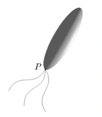
Figure 1: An elongated prolate spheroid with eccentricity 𝝴 = 0.96 providing an approximation of the rod-shaped bacterium.

The second consideration concerns Stokes flow. Stokes flow is defined as a type of motion where the speed of flow is extremely low and the effect of viscosity is very strong due to the viscous forces being much greater than the inertial forces. (Batchelor, 1967). In fluid dynamics, this is represented by a very small Reynolds number Re defined by

Re = Uaρ/μ

where U is the typical velocity of the fluid motion, ρ is the liquid density, a is the typical length scale and µ is the dynamic viscosity of the liquid. Since the swimming speed U is very low and its characteristic dimension a is extremely small, the Stokes approximation is usually adopted for describing the motion of microorganisms (Koiller et al, 1996). It follows that the fluid motion generated by swimming rod-shaped magnetotactic bacteria is governed by the Stokes equation and the equation of continuity:

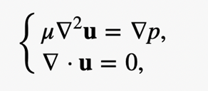
where u is the velocity of the flow and p is its pressure. For understanding the dynamics of swimming magnetotactic bacteria, it is necessary to have mathematical solutions of the Stokes flow created by both the translation and rotation of a rod-shaped body in an infinite expanse of viscous and incompressible fluid. In other words, the analytical solution to the equation above must be in the condition where the fluid velocity u coincides with the bounding surface of a swimming magnetotactic bacterium at each of its points and u approaching 0 far away from the swimming bacterium.

The mathematical solution of a three-dimensional Stokes flow driven by translating an elongated polate spheroid with its eccentricity 0 < (1 – ε) ≤ 1 at an arbitrary angle of attack γ, the angle between the direction of the translating velocity v and the symmetry axis z of a rod-shaped bacterium is required to describe the swimming motion of a rod-shaped bacterium, sketched in Figure 2.

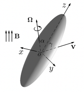
Figure 2: Translation of a rod-shaped bacterium at an arbitrary angle of attack T with the velocity V, where cartesian coordinates (x,y,z) are attached to the bacterium’s body. Rotation of a rod-shaped bacterium with an arbitrary angle alpha and the angular velocity Ω under the influence of an externally imposed, time-dependent magnetic field B.

Adopting the Papkovich-Neuber formulation (Papkovich, 1932; Neuber, 1934), the flow velocity u can be written in the form

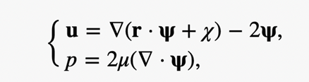
where r is the position vector, Ψ, a vector harmonic function satisfying ∆Ψ² = 0, and x a scalar harmonic function satisfying ∆x² = 0. Both Ψand x can be obtained by using the expansion of prolate spheroidal harmonics (Kong et al., 2012), which will not be covered in this paper due to its relevance and complexity.

The third assumption is made concerning the drag on a moving bacterium. The drag force D_B on a swimming rod-shaped bacterium can be expressed as

D_B=∫_S^ f^t  dS

Where ∫_S denotes the surface integration over the bounding surface S of the bacterium, f^t in tensor notation is

f_i^t=(-p^t δ_{ij}+2μσ_{ij}^t ) n_j

With δ_ij being the Dirac delta function, n_j being unit normal at the bounding surface S and

σ_{ij}^t=1/2 ((∂u_i^t)/(∂x_j )+(∂u_j^t)/(∂x_i ))

Evaluating p^t and σ_ij^t at the outer surface ξ = ξ₀ of the bacterium, where ξ ∊ [ξ₀, ∞) is the radial coordinate characterizing oblate spheroidal surfaces, integrating over its bounding surface S gives the drag force D_B

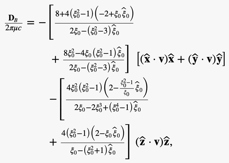
Lastly, torque also needs to be considered when modelling MTB’s motion. One needs the mathematical solution of a 3D Stokes flow driven by rotating bacterium with the angular velocity Ω at an arbitrary angle alpha as depicted in Figure 2. Suppose that a bacterium is rotating with the angular velocity Ω in the form

where 𝝰 and 𝝱 specify the direction of Ω in the cartesian coordinates (x,y,z).

Apart from the special case with 𝝰 = 0, the Stokes flow is fully three-dimensional.

The viscous torque T_B acting on the rotating bacterium can be expressible as

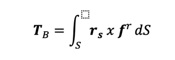
Where r_s denotes the position vector for the bounding surface S of the bacterium and the viscous force f^r on the surface S is given by

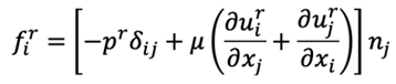
With the velocity u^r_i and p^r evaluated at the bounding surface ξ = ξ₀, of the bacterium.

The torque in cartesian coordinates (x,y,z) is denoted with  

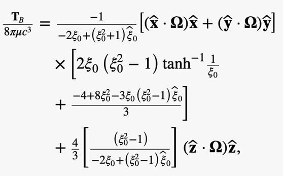
which is valid for arbitrary rotating vector Ω.
Figure 3 shows the variation of the viscous torque with the size of eccentricity 𝝴 for 𝝲 = 45^o, indicating that the dynamics of swimming rod-shaped bacteria would differ from that of spherical-shaped bacteria.

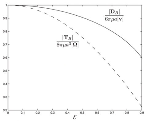
Figure 3: The scaled drag force and the scaled viscous force torque as a function of eccentricity 𝝴 for 𝝲 = 45^o.

Once those factors are taken into account, one can compile all the assumptions necessary to use this specific model. Under the assumptions that 1) the geometry of a rod-shaped magnetotactic bacterium can be described by an elongated prolate spheroid, 2) the body of rod-shape magnetotactic bacteria is non-deformable, 3) interaction between different magnetotactic bacteria during their swimming motion is weak and can be negligible, 4) the translation and rotation of magnetotactic bacteria are powered by the rapid rotation of helical flagellar filaments at a fixed point P which may be modelled a driving force F_B in the body frame

where ω₀ is the frequency of flagellum rotation while F₁₂, F₃ and may be regarded as simple parameters, 5) the inertial effects of swimming rod-shaped magnetotactic bacteria are small and negligible, and 6) the initial phase of growing magnetic moment in a magnetotactic bacterium can be described by

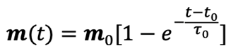
where m is parallel to the symmetry axis of the magnetotactic bacterium, m₀ denotes the magnetic moment in the lim_t→∞, and τ₀ represents a parameter controlling the growth rate of the magnetic moment.

A rod-shaped magnetotactic bacterium swims under the combined action of a propel force F_B , a viscous drag D_B, a viscous torque T_B, and an externally imposed rotating magnetic field B. Newton’s second law states that the rate of change of the momentum must be equal to the sum of all external forces acting on it can be derived into

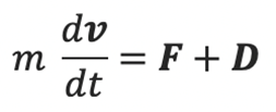
where F and D are the propel and viscous forces. Upon neglecting inertial effects because the mass m of a rod-shaped magnetotactic bacterium is extremely small (around 9.5×10^-16kg), we may rewrite the equation above as

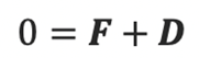
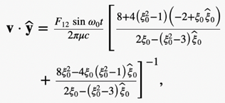
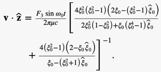
The equations for the propelling force F_B with the drag force D_B above can be used to solve Newton’s second law with the neglection of the magnetotactic bacterium’s mass to obtain the three velocity components in the body frame of the reference.

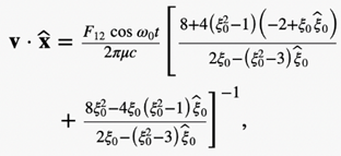
Hence, the swimming motion of rod-shaped MTB in a viscous liquid under the influence of an externally imposed, rotating magnetic field can be modelled using mathematical identities. In fact, a set of 12 differential equations can be used. These differential equations are included in the appendices; however, their derivation will not be covered due to their complexity (Cui et al., 2012).  This model provides scientists with a deeper understanding of the specifically designed motion of MTB in their environment.

Differential Equations Modelling MTB’s Helical Motion

The first three differentials relate to the velocity v_L:

The next three concern the position vector R:

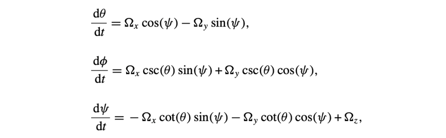
Three of them are for the Euler angles (θ, Φ, Ψ):

The last ones are for the rotation vector Ω:

All equations sourced from (Cui et al., 2012)

[1] The information comes from a lecture handout from Uppsala University. It can be found here: https://www.teknik.uu.se/digitalAssets/386/c_386360-l_3-k_disorder_intro.pdf

[2] This lecture handout is provided by the Good Will Group. It can be found here: http://goodwin.chem.ox.ac.uk/goodwin/TEACHING_files/l1_handout.pdf