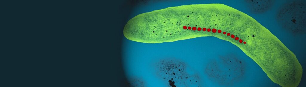
Figure 1: Magnetotactic Bacteria (Perduca, 2016).

Abstract

Magnetotactic bacteria (MTB) are unique aquatic microaerophiles that can align and move in the direction of the Earth’s magnetic field. In this paper, the basic physical properties of magnetosomes, some mechanisms, such as magnetotaxis, and phototaxis, involved in the MTB’s motion, and the role of active magnetotactic sensing are described as evolutionary developments leading to magnetotactic bacteria’s survival. Moreover, it is shown that a good understanding of the fundamental principles of fluid flow and Brownian motion is required to grasp the adaptations and advantages behind MTB propulsion. The important role of the cytoskeleton in providing mechanical stability to magnetosome chains, and the advantages of magnetic alignment to follow optimal oxygen concentrations, are emphasized. Finally, an in-depth investigation of the oxic-anoxic layer in water columns is made, showing the complex dynamics that describe the movement of this layer due to several environmental factors. These various mechanisms and environmental factors reveal that MTB have adapted highly sophisticated sensing and motility mechanisms, that have provided them with remarkable survival advantages in their highly mobile biotope.

Key words: Magnetotactic bacteria, magnetic fields, sensing, motion, oxic-anoxic interface

Introduction

Humans tend to get lost quickly, even when using Google Maps or any other GPS. While some people tend to struggle with directions much more than others, no one can perfectly navigate every time even with our current navigation solutions. Would it not be great if everyone had their own compasses included in their bodies? Sadly, this gift has not evolved in humans. Conversely, magnetotactic bacteria (MTB), some of the most diverse, and widespread prokaryotes found on Earth, developed higher navigation systems. These prokaryotes are characterized by a unique organelle, their compass, called the magnetosome. This biomineralized magnet allows them to be motile and perfect their navigation (Lefèvre & Bazylinski, 2013). These prokaryotes were independently discovered by Salvatore Bellini in 1963 and Richard Blakemore in 1975. Bellini, while being part of an Italian team studying water quality, discovered certain bacteria that consistently collected on the same side of the water droplets. He used a magnet to stimulate them and concluded that they were magnetosensitive. Later, Richard Blakemore published an observation where he noted that there was a microorganism whose swimming direction was altered by the presence of a magnetic field. He coined this response as magnetotaxis (Fernanda & Daniel, 2018). The discoveries made by the two researchers mentioned above proved to be significant to many other research fields such as microbiology, geology, mineralogy, crystallography, and many more.

In the following sections, this paper will investigate the physical properties and interactions of magnetotactic bacteria with its environment. It will begin by discussing the magnetic behaviour of the bacteria and its interactions with geomagnetic field lines. Furthermore, adaptations such as flagella in MTB and the advantage of magnetosome chain alignment will be explained by various scientific concepts, such as the Navier-Stokes equation for fluid flow and Brownian motion. The role of different intercellular components that allow alignment and provide stability to the magnetosome chain, will be elucidated. Finally, this paper will cover the principles behind the mobility of the environment in which magnetotactic bacteria thrive, highlighting the reason why the bacteria in question need efficient transport mechanisms.

Magnetotaxis

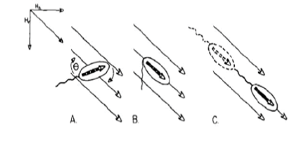
Magnetotaxis evolved in bacteria during the Archean, a period dating back to 4 billion years, becoming a significant physiological feature in magnetotactic bacteria (Fradin, 2013). It is the response in magnetotactic bacteria to external magnetic fields that allows them to orient their direction of navigation with these geomagnetic field lines (Fernanda & Daniel, 2018). Magnetotactic bacteria contain many organelles, one of which is unique to gram –negative bacteria. This organelle is the magnetosomes presented as darker arrows inside Figure 2. These are made of iron oxide or iron sulfide crystals enclosed in a membrane, and their primary function is related to magnetotaxis. These organelles act as permanent magnets, providing the bacteria with their own little internal compass. The purpose of these magnets is to help the bacteria navigate in their biotopes.

Figure 2: Magnetotactic bacteria demonstrating magnetotaxis [Adapted from Dasdag, 2014].

In the northern hemisphere, they follow Earth’s magnetic field lines towards the South, where there are lower oxygen concentrations. In the southern hemisphere, their compass-like abilities direct them towards the North, where there is less oxygen once again (Fradin, 2013). At the equator, magnetotactic bacteria from both hemispheres can be found because there is no magnetic North pole oriented up or down (Fradin, 2013). These responses to magnetic fields are very helpful for scientists who want to study bacterial motion. Experimental and theoretical studies have shown that magnetotactic bacteria swim in a cylindrical helix trajectory (Fradin, 2013). Magnetosomes generate a magnetic moment which interacts with the geomagnetic field lines. This interaction results in torque, from which stems magnetotaxis and the ability to self-navigate. The most stable configuration of these magnetosomes would be a ring. However, in nature, they are observed as a line kept in place by the cytoskeleton (Fernanda & Daniel, 2018). The linear conformation of the magnetosome allows it to behave like a proper compass needle. The magnetic properties of the magnetic nanoparticles within the magnetosomes depend on the size of the particles. For smaller nanoparticles whose size ranges in the single magnetic domain (atom alignment generates a uniform unidirectional magnetic moment in one direction, which can be achieved within 3-50nm size), the random changes in orientation of small particles due to thermal energy result in their unstable magnetic moment (this phenomenon is called superparamagnetism), which is undesired for effective navigation. However, if the size of nanoparticles is increased but remains within the single magnetic domain, the direction-specific energy increases, creating an energy barrier that maintains a fixed direction for magnetic moment. This increases their stability and sensitivity to external magnetic fields (this occurs when sizes are within 30-120nm, which matches the size of a magnetosome), which is optimal for navigation (Fernanda & Daniel, 2018; Newell, 2009).

Magnetic Moment

Many techniques are used to determine the bacterial magnetic moment that is generated from their magnetosomes, shown in black in Figure 3. The magnetic moment determines the magnetic strength and orientation of the magnetosome. The magnetic electron holography technique allows observations of the magnetic flux lines created by the aligned magnetosomes (Fernanda & Daniel, 2018). Electron holography permits scientists to determine the amplitude and phase of a signal distribution by comparing it to a known reference, therefore allowing it to image magnetic structures (Madan et al., 2019). It is possible to calculate the magnetic moment (M) of a magnetosome chain with the equation M = nV_indM_V, where n is the number of particles in the chain, V_ind is the volume of each particle assuming they are all equal, and M_V is the magnetic moment per unit volume of magnetic material. For example, a chain composed of 22 particles of magnetite with volumes of 1.25 x 10^-16 cm³ each with M_V = 480 × 10^-3 Am²/cm³ has a magnetic moment M = 1.3 × 10−15 Am². This method can be used to count how many magnetosomes are in a train, but it is not applicable to live bacteria or larger organisms with many more magnetosomes.

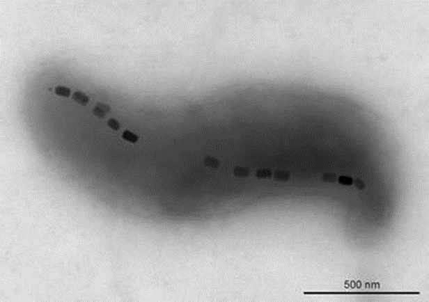
Figure 3: Transmission electron microscopy of the magnetotactic bacterium Magnetovibrio blakemorei strain MV-1 showing a single chain of prismatic magnetite magnetosomes (Fernanda & Daniel, 2018).

Assuming that magnetotactic bacteria behave as paramagnetic particles, the orientation that magnetotactic bacteria have in space when swimming can be described by the average of cosθ, where θ is the angle between the magnetic field and the bacteria’s velocity. Cosθ is a function of the magnetic-to-thermal energy ratio: Cosθ = L(MH/kT) = Coth(MH/kT), where M is the bacterium magnetic moment, H is the magnetic field intensity, k is the Boltzmann constant, T is the absolute temperature, and L(x) is the Langevin function: coth(x)—1/x (Hall, 2023). When MH/kT ≈ 10, L(x) ≈ 0.9, it means that the bacterial trajectory is well oriented to the magnetic field direction (Hall, 2023). The drawback of these calculations is that they can only be used to analyze the trajectory of a single bacterium, not the average of multiple bacteria. Another way that the magnetic moment of these organisms can be analyzed is by using a SQUID magnetometer – a superconducting quantum interference device, which can be used for detecting and measuring magnetic fields generated by current (Hall, 2023). This instrument determined an average magnetic moment of 1.8 ± 0.4 × 10^-12 emu for bacteria from natural sediments. Magnetic moment is a key feature that allows magnetotactic bacteria to interact with and move throughout their environment.

Light Response and Phototaxis

The movement of magnetotactic bacteria also depends on the presence of light because they respond to different wavelengths and light intensity. A study on multicellular magnetotactic prokaryotes has shown that negative phototaxis is observed when these organisms are illuminated with high-intensity UV light of 365 nm in wavelength, as well as violet-blue light of 395–440 nm wavelength of about 80 W m^-2 intensity, and blue light of around 450–490 nm wavelength of about 200 W m^-2 intensity. This study also concludes that there was no negative phototaxis at very low light intensities (Fernanda & Daniel, 2018). Phototaxis is the response in the form of movement to external light stimulus by an organism. Negative phototaxis means that the bacteria respond to the light by moving away from the direction of increasing light intensity (Dey). No phototaxis was observed in response to longer wavelengths (Hall, 2023). Photokinesis, which is a change in velocity in response to light, was also observed in these bacteria. Green light (517 nm, 0.46 W m−2) decreased the velocity of the organisms, while red light (628 nm, 0.16 W m−2) increased the velocity. It was shown that photokinesis is affected by the combined presence of monochromatic light and a constant magnetic field. Furthermore, photokinesis can be canceled by the presence of radio-frequency electromagnetic fields that oscillate at the Zeeman resonance frequency that the constant magnetic field is associated with (Fernanda & Daniel, 2018). This is because photokinesis depends on the presence of a constant magnetic field, as well as monochromatic light. The Zeeman frequency refers to the splitting of a spectral line into two or more components of light when it is in a magnetic field (“Zeeman Effect”, 2011). The light source will no longer be monochromatic since some atomic levels will split into several levels with different energies, so photokinesis cannot occur. This demonstrates that a radical pair mechanism is involved in magnetotactic bacteria as well, which is a magnetoreception mechanism that migrating birds use. Therefore, magnetotactic bacteria can also sense Earth’s geomagnetic field using light.

Magneto-Aerotaxis: Magnetically Assisted Aerotaxis

A major advantage of directing movement along a magnetic field is the increased ability of MTB to rapidly reach optimal oxygen concentrations (Smith et al., 2006). The main feature of orienting to magnetic field lines is that, unless located close to the equator, they contain a significant vertical component that allows MTB to move downwards away from high oxygen concentrations.

The benefit of magneto-aerotaxis was quantified in an experiment by Smith et al., where vertical displacements of wild type (WT) Magnetospirillum magneticum AMB-1 were compared to those of an engineered mutant (which could not produce magnetosome chains) DmagA1 AMB-1, in an oxygen-exposed environment. In the experiment, AMB-1 cells were placed and distributed inside a cuvette and were then exposed to oxygen which would progressively dissolve inside the liquid. In this way, AMB-1 cells would move toward the bottom of the cuvette to remain in low-oxygen levels required for optimal growth. A mathematical model and simulation were also used to compare experimental evidence. As shown in Figure 4, which plots of the optical density towards the bottom of the cuvette (apparatus shown in Figure 5), which indicates AMB-1 cell concentration over time, the experimental curve (black) is close to the simulated curve (grey), allowing conclusions to be based on the parameters of the mathematical model. Here, the parameter of interest was the critical oxygen concentration at which AMB-1 cells would start moving to lower oxygen concentrations. It was concluded that migration was faster in WT cells, and that migration rate in WT increases with magnetic field strength, as can be shown in Figure 4. The most interesting result is that the critical oxygen concentration required for AMB-1 cells to swim to lower oxygen concentrations is 66 times higher in WT than in Dmag-A1 cells, which is also significantly higher in WT cells in stronger magnetic fields. This result shows that sensitivity to oxygen concentrations is enhanced with magnetotaxis, which provides a significant advantage, considering that high oxygen concentrations is an important factor limiting the growth of anaerobes and microaerophiles (such as AMB-1) MTB. One reason for this result is that, considering the fact that mutant AMB-1 are oriented randomly when traveling in a particular direction along an axis (e.g. downwards towards low oxygen conc.), the average speed of the mutant is half that of the aligned WT bacteria. This would allow higher migration rates in WT AMB-1 cells. However, this does not seem a plausible explanation for the fact that oxygen sensitivity is 66 times greater in WT than in mutant cells. This suggests that the mechanism behind magnetic advantage is of nature beyond the physical properties of magnetosome chains, and possibly involves biochemical processes that depend on magnetosomes and their alignment to external magnetic fields (Smith et al., 2006).

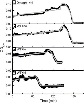
Figure 4. Optical density (indicative of bacterial density) WT and mutant AMB-1 cells at the bottom of the cuvette along time (min). The term “no” means no magnetic field applied, “lo” and “hi” mean low and high magnetic field strength (Smith et al., 2006).

Figure 5. Experimental apparatus for applying a vertical magnetic field and detecting bacteria at the spectrometer window (Smith et al., 2006).

Sensing Mechanism

The mechanism behind the navigation of magnetotactic bacteria along the magnetic field has been explained by two different models. Some researchers support the idea that their magnetotactic behavior is the result of passive alignment with the magnetic field, while others argue that it is due to the active sensing of the magnetic force (Zhu et al., 2014). Some state that the active sensing mechanism is unnecessary given calculations showing that the interaction of dipole moment and the geomagnetic field is strong enough to “overcome rotational diffusion of the cell orientation induced by thermal noise in the medium” (Kalmijn, 1981). In contrast, Greenberg et al. suggest that a receptor mechanism for the sensing of magnetic field may be used instead (Greenberg et al., 2005). To confirm this, Xuejun Zhu et al. have developed a microfluidic device to observe the swimming patterns and magnetotactic behavior of Magnetospirillum magneticum AMB-1 cells at the single-cell level in a range of magnetic fields.

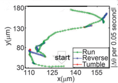
Figure 6: Swimming pattern of cell. Every point represents an interval of 0.05 seconds (Zhu et al., 2014).

Time-lapse microscopy was used to track the swimming paths of AMB-1, and observations showed the bacteria sometimes backtracked before resuming its forward motion (Figure 6). This behavior is defined as “run and reverse” and does not always occur simultaneously. In fact, a brief adjustment period was observed from time to time that allowed the bacteria to reorient itself in an unpredictable manner. This transition state is defined as tumble. However, it is important to note that a reversal does not always take place in the event of a tumble. It may occur that the bacteria resume their forward or reverse swimming paths: run-tumble-run and reverse-tumble-reverse (Zhu et al., 2014).

The experiments showed that active sensing does exist in magnetotaxis and that Amb0994, the only methyl-accepting chemotaxis proteins (MCP) in the magnetosome island lacking an extracellular domain, functions as the magnetic receptor (Philippe & Wu, 2010).

The removal of Amb0994 from the AMB-1 kept the synthesis and alignment of its magnetosomes fully intact, and the swimming patterns remained like the ones observed in wild type cells. However, the cells were unable to align themselves with the magnetic field. Under the influence of a magnetic field of 1.0 mT, wild type cells’ behavior was normal, in contrast to mutated cells without Amb0094, where a randomized swimming pattern was observed (figure 7).

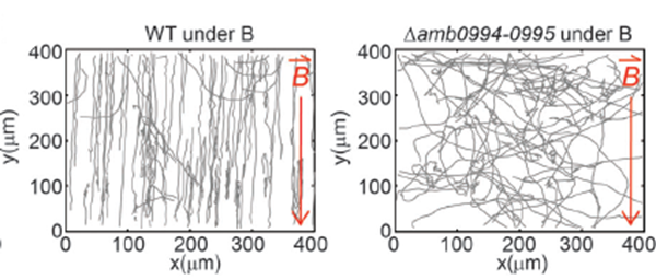
Figure 7: Trajectory of cell with and without Amb0094 under a 1.0 mT magnetic field (Zhu et al., 2014).

Furthermore, the motion time under an external magnetic field of 1.0mT saw a massive drawback of 46.81%, 48.05%, and 45.0% compared to wild type cells in the running, reversal, and tumbling states respectively. All these observations demonstrate that the deletion of Amb0094 MCPs affects the cell in a way that disrupts its response to an external magnetic field, therefore suggesting that Amb0094 is responsible for the sensing of magnetic fields (Zhu et al., 2014).

To further validate Amb0094, Amb2196 was used to compare the cell’s behavior under the same conditions of 1.0mT. This MCP shared the highest similarity with Amb0094 at 97% (Zhu et al., 2014). However, the run and reverse time of the Amb2196-lacking cell yielded very similar results to the wild-type cell, which confirmed that Amb0094 played an important role in sensing magnetic fields.

Active angle sensing in AMB-1

For magnetotaxis, the torque depends on the angle between the magnetic dipole moment inside the cell and the external magnetic field. An increase in this v-B angle generates a higher torque, which increases the probability of tumbling. A larger v-B angle would increase these odds since the cell is drifting away from the magnetic field and would have to tumble to reorient itself at the correct alignment. This negative correlation between the v-B angle and the likelihood of a tumble can be further illustrated with the mean run-time of the cell. In fact, as shown in Figure 8, the higher the v-B angle, the lower the average run-time. The run-time is stable and increases if the cell is aligned with the magnetic field, which allows it to maintain its forward swimming state for a longer period. It is worth noting that the correlation between the v-B angle and the reverse-time is less significant given the already very brief duration of the reverse state (figure 8) (Zhu et al., 2014).

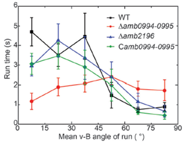
Figure 8: Relationship of the mean v-B angle with the run-time of a wild type cell (black) (Zhu et al., 2014).

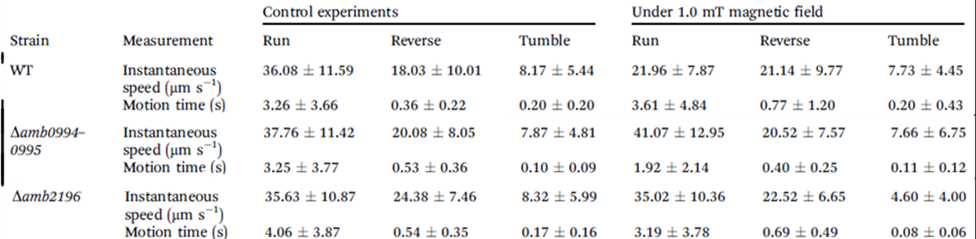
Figure 9: Motion time in seconds of mutated cells lacking amb0094 or amb2196 and wild type cells in control experiments and an external magnetic field of under 1.0 mT (Zhu et al., 2014).

This correlation was also studied in mutant AMB-1 cells lacking Amb0094 or Amb2196. In a cell lacking Amb2196, the negative correlation between the v-B angle and the run-time followed the trend of that in wild type cells, that is, a pronounced drop in run-time with increasing v-B angle. However, in mutant cells lacking Amb0094, the run-time was independent of the v-B angle. Rather than decreasing with the v-B angle, it increased between 15^o and 45^o before a slight decrease in run-time (figure 8). These results pointed out that the active sensing of magnetic fields was involved in the magnetotaxis of AMB-1, and that Amb0094 functioned as the active magneto-receptor (Zhu et al., 2014).

The Passive Alignment model and its Shortcomings

The passive alignment model follows the mechanism of a compass, where the rotational motion of the bacteria cell is influenced by magnetic torque and thermal fluctuations. Given the fixed position of the chain of magnetosomes, the cell orients itself passively toward the magnetic field while in motion and therefore behaves as a self-propelled magnetic compass needle that migrates along geomagnetic field lines (Frankel & Bazylinski, 2006).

The passive alignment model implies that the distribution of the cell’s direction for all strains should be given by the Boltzmann distribution p(θ) = Ae^-Em/kT, where E_m is the magnetic field, A is the normalization constant, k is the Boltzmann constant, and T is the temperature. E_m is given by -mB|cosθ|, where m corresponds to the cell’s magnetic dipole moment, B the external magnetic field, and θ the angle between the cell’s polar direction and B. Since the v-B angle, Φ, is measured by projection into the 2-D observation plane, the average angle is as follows in Figure 10:

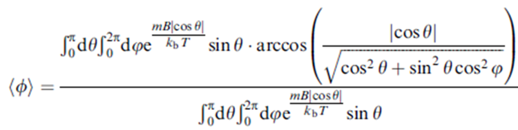
Figure10: The average angle equation [Adapted from (Zhu et al., 2014)].

However, the results yielded experimentally were higher than the predicted v-B angle from the passive alignment model. The effective temperature, T_effective, the temperature for which the experimental data was used to fit the passive alignment model was around 340 times larger than the room temperature: T­_-effective = 3400K compared to 301K. This temperature provides an approximation of the overall strength of the noise caused by the cell’s active reorientation. This large deviation indicates that the active reorientation of the cell creates considerably more noise than the temperature variation of the environment (Zhu et al., 2014).

Furthermore, as opposed to experimental results obtained in a magnetic field of under 1.0mT, measurements showed that for a higher magnetic intensity, such as over 5.0mT, wild type and mutated cells showcased the same magnetic response. This suggests the passive alignment of the cell becomes more important and meaningful compared with the active sensing mechanism. Altogether, both passive and active models describing the magnetobehavior of AMB-1 are valid. As seen, Amb0094 functions as the active magneto-receptor and plays a significant role in the navigation of the cell at low magnetic intensities. On the other hand, passive alignment becomes much more relevant under high magnetic intensity fields when it can overcome the active motion of the cell.

Fluid Dynamics: Constraints on Bacterial Propulsion

To obtain a deeper understanding of the movement of magnetotactic bacteria and elucidate the advantages of the specific behaviors and structures they can have, it is important to explore the fundamental concepts of fluid flow and Brownian motion and how they apply in a micron range. Fluid flow is a complex dynamics problem that includes several forces that may vary depending on the situation. However, there remain fundamental internal forces that are generated by the interactions of the fluid’s particles and related to characteristic properties of the fluid, such as its viscosity. All so-called incompressible Newtonian fluids (including gases, liquids, and even solids – e.g. glaciers that move over time in frozen rivers), can be modeled by the Navier-Stokes equation, given by

ρ (∂u ⃗)/∂t+ρ(u ⃗⋅∇u ⃗ )=-∇p+η(∇∙∇u ⃗ )+f ⃗

Where ρ is the density of the fluid, η is the fluid’s viscosity, u is the velocity field of the fluid, and where p denotes pressure.

Would you like to know?

If you would like to understand how the non-dimensionalized form of the Navier stokes equation is obtained (and that it is actually equivalent to the form that was started with), check out this video: https://www.youtube.com/watch?app=desktop&v=pucOcvFAkiw

Although this equation seems complex, it is only a rewritten form of Newton’s second law, where the left-hand side is equivalent to the product of the fluid’s mass and acceleration ρ(du/dt). This last term is separated into two terms: ρ(du/dt) represents the change in speed of a fluid particle over time, and ρ(u∙∇u) represents the change in the concentration of the flow’s velocity field lines over a fixed infinitesimally small volume dxdydz. The right-hand side of the equation comprises all the forces that apply on the same infinitesimally small volume. Here, -∇p is the pressure gradient, which equals the average of all normal forces on the dxdydz volume that causes a deformation of that volume.  η(∇∙∇u) represents the shear stress that this dxdydz volume experiences, which is caused by the friction of the fluid on that volume, being proportional to the fluid’s viscosity η. Additionally, f is any other external force that may apply in the system. Although this form of Navier-Stokes equation is instructive of fluid flow, it can be rescaled to allow its use with measurable variables, and to adapt to the low scale that applies in the micron range. This rescaling is essentially a change in coordinate systems and allows to adapt to characteristic length Lo (e.g. the length of a magnetotactic bacteria), velocity vo (of a magnetotactic bacteria), and To (may equal Lo/vo, or another value if there is a movement boundary around the fluid, which affects the global displacement of a single bacteria). This rescaling leads to the following equation:

Re(L_o/v_o )  (∂(u') ⃗)/∂t+Re((u') ⃗⋅∇'(u') ⃗ )=-∇'p'+η(∇'∙∇'(u') ⃗ )+f ⃗'

Here, Re is the Reynolds number, which is a unitless ratio of inertial forces to viscous forces. Low Reynolds numbers (≤ 2100) indicate that a flow is predominantly laminar (more viscous and flow lines parallel) and high Reynolds numbers (≥ 2100) indicate the predominance of turbulent flow (more “fluid”/less viscous and curved non-parallel flow lines) (Rehm, 2008). In water at a microscopic level, the Reynolds number is in the range of 10^-7 – 10^-3, where laminar flow predominates. Consequently, the Navier-Stokes equation becomes:

0 =-∇'p'+η(∇'∙∇'(u') ⃗ )+f ⃗'

Would you like to know?

To understand the result and implications (i.e. the reversibility of movement at low Re and non-reciprocal motion) of this final equation in a little more detail, check out this video on movement at low Re numbers: https://www.youtube.com/watch?v=BMwy_9y2TWI

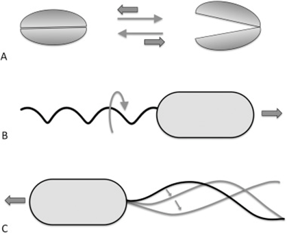
This eliminates the inertial terms in the equation so that inertia does not matter, meaning that a body cannot be in motion without the presence of an external force. This can be illustrated by the fact that when a bacteria moves at high speeds with its flagella and then suddenly stops, it stops within a distance of only 0.1 angstroms, which is approximately half the size of a hydrogen atom (Klumpp et al., 2019). This phenomenon constrains the way bacteria must move in their environment (Klumpp et al., 2019). Specifically, motile structures must be designed such that non-reciprocal movement will be generated (Klumpp et al., 2019).

Figure 11: Reciprocal (A) and non-reciprocal (B, rotating flagellum, and C, sperm cell flagellum motion) movements in the micron range. Movement A does not go anywhere, while movements C and B are propulsive.

Reciprocal movement is a cyclic motion that is comprised of two identical and opposite movements, such as those generated by the continuous opening and closing of scallop shells (Palagi et al., 2017). If scallops were reduced to a microscopic size comparable to bacteria, they would not be able to move, as the opening of their shell displaces them in the opposite direction of its previous motion (see Figure 11) (Palagi et al., 2017). This constraint is why the helical structure of flagella is chiral, such that non-reciprocal movement can be generated as flagella rotates clockwise or counterclockwise to allow bidirectional movement (Palagi et al., 2017). Flagella are important structures in marine MTB, as these need to move in along the oxic-anoxic interface, which displaces over time along chemically stratified sediments or water columns. Marine MTBs can possess up to tens of thousands of flagella to increase their chances of consistently finding locations with optimal conditions for survival (Zhang & Wu, 2020). An example of MTB with highly adapted flagellar apparatus is the M.massalia strain, which possesses bundles of 7 flagella that are each sheathed to generate a propulsion force nine times stronger than obtained with unsheathed flagella (Zhang & Wu, 2020). It is also thought that this sheath, which is similar in other MTB strains, serves as a protective layer that prevents damage in the structural components of flagella due to sediments in chemically stratified environments, suggesting that this sheath is a result of adaptive evolution (Zhang & Wu, 2020). The complexity of the flagellar structure in MTB strains M.massalia  and M. marinus is indicated by the fact that they possess the largest number of flagellin (flagellar synthesis genes) genes, which suggests a high level of adaptations for optimal motile function (Zhang & Wu, 2020). The most striking feature is that magnetotactic include some of the fastest bacterial microorganisms, achieving speeds of 300 µm/s in M.massalia to 500 µm/s in  magnetic cocci for bacterial sizes of only ~1.3 300 µm (Bente et al., 2020; Zhang & Wu, 2020).

Overcoming Brownian Motion

Although the self-propulsion of MTB by flagellar motion provides highly adaptive motile capacities, they must still be composed of diffusive and rotational forces that are a direct consequence of Brownian motion (Klumpp et al., 2019). Brownian motion is the random motion of small particles in suspension that undergo collisions with surrounding particles. In this case, bacteria can be considered Brownian particles that undergo collisions with solvent molecules. Here, mathematical details of Brownian motion are spared, but it is important to note that this is used to describe the diffusive motion of particles. In diffusive motion, the mean square displacement is proportional to time and temperature and is inversely proportional to the viscosity of the fluid (more viscous à more laminar flow à weaker diffusive movement) and the size of the particle (increasing size leads to increased friction). In the micron range, the relative importance of self-propulsion and diffusion (resulting in Brownian motion) varies in time, and the interplay of these motions generates a movement pattern described in Figure 12.

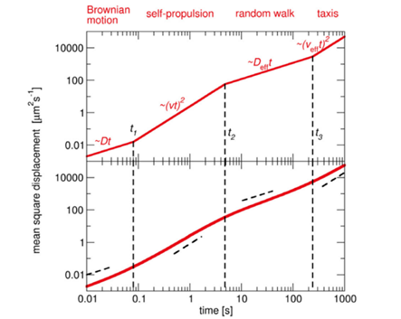
Figure 12: Mean square displacement over four-time domains. The upper plot is a theoretical curve of such movement pattern, and the bottom plot was obtained experimentally from a particle undergoing run-and-tumble motion (Klumpp, Lefèvre et al., 2019).

The ratio of self-propulsion to Brownian motion can be described by the Peclet number, which is:

Pe=Lv/D  

Where L is a variable length based on the distance travelled by a bacterium from a given point, v is the speed of the bacteria, and D is the diffusional coefficient. Large Peclet numbers (generally when Pe ≫ 1) indicate that self-propulsion dominates, while small Peclet numbers (Pe ≪ 1) indicate that Brownian motion dominates. At the beginning of the motion pattern,  L is much smaller than the diffusion coefficient, indicating that Brownian motion dominates. However, this only applies for a short period of time, given the high velocities of MTB and typical diffusion constant of 0.1 µm²/s. After this short timescale, self-propulsion dominates, but over long distances, rotational diffusion changes the orientation of the bacterium, effectively generating an overall diffusive movement. This prevents the bacterium from maintaining its directed movement and gives rise to random walks, where the orientation remains constant for some time until direction becomes randomized, leading to diffusive movement over longer time scales. Then, depending on the nature of a stimulus (mechanical, chemical, gravitational, etc.), a taxis, which is the bacterium’s action of directing its motion due to an environmental signal, may be performed to control motion. One main advantage of MTB is that their continuous alignment with the Earth’s magnetic field minimizes the effects of Brownian motion. In fact, the ratio of the combined magnetic moment of MTB with the external magnetic field to the thermal energy that causes Brownian motion which randomizes magnetosome direction, MB/k_BT (where k_B is the Boltzmann constant, T is temperature, M is the magnetic moment, and B is the external magnetic field), is of importance, and determines the alignment of the magnetosome chain to the external magnetic field according to the Langevin equation

cos⁡(θ)=coth⁡(MB/(k_B T))-(k_B T)/MB

Where θ is the angle of alignment (Satyanarayana et al., 2021). Typically, the energy of alignment in Earth’s magnetic field with magnetosomes in MTB at normal temperature is -7.6 k_BT, which allows a parallel orientation (Klumpp et al., 2019). The MTB’s ability to passively overcome the randomizing effect of thermal energy is a significant advantage that reduces MTB’s three-dimensional search for optimal oxygen concentrations from a one-dimensional search (Smith et al., 2006). In fact, MTB alignment with the magnetic field is a more energy-efficient motile strategy as compared to the run-and-tumble motion of non-magnetotactic bacteria, and the average speed at which MTB travel towards a point of interest corresponds to a significant portion of its forward speed (90%), indicating rapid displacements towards optimal locations (Mann, Sparks, & Board, 1990).

Cytoskeleton and Mechanical Stability of Magnetosome Chains

A universal rule is that any closed system (that can exchange energy with surroundings) will naturally adopt the configuration that minimizes its energy. This stems directly from the second law of thermodynamics, and magnetosome chains do not make an exception to this law. To passively orient to the Earth’s magnetic field, MTB must have linear magnetosome chains that can align to magnetic field lines. However, a stable configuration of magnetosome chains is rings, which increases magnetic interactions between magnetosomes (Kiani, Faivre, & Klumpp, 2015). In fact, a simulated experiment on magnetosome chains shows that rings occur at the same frequency as linear formations, as shown in the first band of Figure 13 (Kiani, Faivre, & Klumpp, 2018). These results are also supported by experiments performed with isolated magnetosomes (Philipse & Maas, 2002). MTB avoid this problem, as their cytoskeleton acts as a scaffold that holds magnetosomes in place. As can be shown in Figure 13, the magnetosome chains are more linear as the binding energy between the filament and magnetosomes is increased. The components responsible for providing mechanical stability to magnetosome chains are the MamK and MamJ proteins. MamK is an actin filament that is attached to magnetosome chains through the MamJ protein (Scheffel et al., 2006).

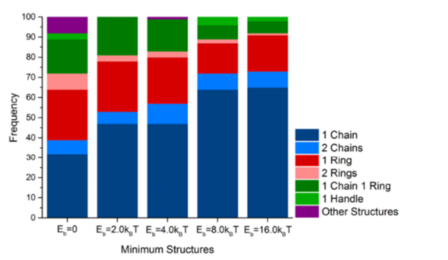
Figure 13: Fraction of configurations observed in the Monte Carlo computer simulations in the absence and presence of different values of the binding potential of the filament (Kiani, Faivre, & Klumpp, 2018).

In the simulated experiment by Kiani et al. and another experiment on isolated MTB by Koernig et al., external magnetic fields with different strengths were applied to magnetosome chains and rotated to determine critical angles at which the chains were disrupted. In both studies, the competition between the magnetosome-magnetosome interactions, and the interactions between magnetosomes and the external magnetic field, were considered. Rotating the magnetosome dipoles increases the interaction energy between magnetosomes until these interactions become repulsive (Kiani, Faivre, & Klumpp, 2018). In the study conducted by Koernig et al., only the magnetic interactions were considered in their theoretical model, and any discrepancy in their measurements was used to determine the stabilizing role of cytoskeletal elements. It was observed that there is an abrupt change in chain alignment when external magnetic field strength reaches 35mT (i.e. the chain does not rotate at 20 mT and 30mT, but is perfectly aligned at 35mT). Also, the fact that magnetosome chains did not rotate below a certain external magnetic strength threshold would not make sense with the theoretical model which predicted a gradual alignment with the external magnetic field. In addition, after a threshold magnetic field strength was applied so that magnetosome chains align perfectly, the chains still align under a weaker external magnetic field strength (i.e. 10 mT). These results suggest a permanent disruption of an assembly that holds the magnetosomes, and accounting for the theoretical model allows us to determine a maximal force of 25 pN that is born by the cytoskeletal elements (namely, MamJ, which holds MamK and magnetosomes). This stability is sufficient to keep magnetosomes in a linear conformation, which enables the magnetosome chain to behave as a compass for optimal navigation.

Magnetotactic Bacteria’s Ideal Biotope

The reason why such emphasis was placed on describing functions that lead to motion is because these magnetotactic bacteria are constantly moving, reorienting themselves, and attempting to reach their ideal biotope to survive. Their ideal biotope is found at the oxic-anoxic interface (OAI) in bodies of water as presented in Figure 14 (Lefèvre & Bazylinski, 2013). The oxic-anoxic interface is the layer of water located between opposing gradients of oxygen and reduced compounds. This type of interface can be found in many aquatic environments such as freshwater, marine, brackish, or even hypersaline. This explains the omnipresence of magnetotactic bacteria on the planet. The presence of the oxic-anoxic zone depends on many physical principles. This section will cover the formation of such a zone, the major factors accountable for the location of this zone, and some events that can cause variations in the position of this interface.

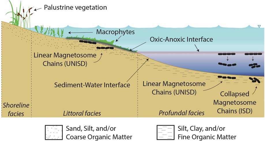
Figure 14: Conceptual model of the OAI presenting the position of magnetosomes relative to the littoral area (elements are not up to scale) [Adapted from Lascu, 2013].

Formation of the Oxic Anoxic Interface

A zone with opposing gradients of oxygen such as the oxic anoxic interface originates from imbalances between organic matter, and oxygen in waters of considerable depth (Weidner et al., 2020). Anoxic zones are sections of the water column that contain extremely low concentrations of oxygen. These sections have a great influence on the magnetotactic bacteria’s position (Weidner et al., 2020). The low oxygen levels found in the depths of the anoxic zones are primarily caused by limited water exchange between bodies of water, and limited ventilation of the deep stratified waters (Weidner et al., 2020). This region is present in all aquatic ecosystems. In some, it is positioned within sediments, while in others, it can start up to several meters before the bottom (Brune, Frenzel, & Cypionka, 2000). This depends on the activity level in the aquatic environment. Towards the upper bounds of this region is located the oxic anoxic interface where waters void of oxygen meet waters containing low concentrations of oxygen. This zone is inhabited by many bacteria because a variety of resources necessary for their function is present. (Brune, Frenzel, & Cypionka, 2000). It follows that this presence of microbiota amplifies the opposing gradients as they perform daily functions. Accordingly, the combination of strong stratifications of the water columns and the presence of bacteria at the interface is responsible for the main contribution to the formation of oxic-anoxic zones.

Influence of Oxygen

What defines the position of the oxic-anoxic zone is the concentration of oxygen in water. Gaseous oxygen has one of the most important roles in the energic situation of organisms. The importance of its presence or absence is amplified in aquatic environments as oxygen has a low solubility in water (Weidner et al., 2020). However, oxygen is not limited to dispersing in water, it can also diffuse in sediments varying with the trophic state of the aquatic body (Brune, Frenzel, & Cypionka, 2000). The different trophic states depend on the amount of biological activity water can sustain. The more activity there is in the water, the cloudier it is because of nutrients and the shallower light penetrates. The OAI will only occur once the light from the surface has decayed. Oligotrophic waters represent the least activity and eutrophic the most activity (Brune, Frenzel, & Cypionka, 2000). Oxygen transport into the sediments will only occur when the OAI is buried under them and will rarely occur if the interface is located higher (Brune, Frenzel, & Cypionka, 2000). Oxygen penetration is controlled by molecular diffusion, and it can be measured with “the slope of the oxygen profile in the diffusive boundary layer” (Brune, Frenzel, & Cypionka, 2000). In other words, it follows Fick’s first law of diffusion stated below:

J=-D_s ϕ  dC/dx

This equation means that the net amount of compound diffusing (J) relies on its motility in a medium, given by the diffusion coefficient (D_s) and the steepness of the concentration gradient (dC/dx). The porosity of the sediment (∅) also must be considered (Brune, Frenzel, & Cypionka, 2000).

Stable Stratifications

Water in most aquatic environments is defined as a stratified fluid. This means that the fluid density increases with the depth of the water (“1 – Fundamentals,” 2002). The variations in the density of water are influenced by the temperature and the salinity of said water according to the following equation (Sherman, Imberger, & Corcos, 2003).

dρ=-αdT+βdS

In this equation, α is the coefficient of thermal expansion and β is the coefficient of saline contraction. Consequently, as temperature increases, the density decreases, and as salinity increases the density increases also. Layers of different densities will rest upon each other because of the buoyancy force that occurs when they are displaced from equilibrium. The buoyancy force is the sum of all the vertical forces placed upon a “piece” of water (Hautala, 2020). It can be described in the following equation.

∑F_b=((ρ_2-ρ_1)/ρ_1)  g

Correspondingly, the buoyancy force is dependent on the gravitational acceleration (g) and the percentage of the density difference of the piece of water (ρ₂) compared to the surrounding water (ρ₁) (Hautala, 2020). Furthermore, a downward displacement of water will generate a buoyancy force towards the surface and vice versa (Hautala, 2020). Based on those principles, it follows that they do not usually mix, and the oxic-anoxic interface will usually move as one unit across the layers if general disturbances occur (Valerio et al., 2019). This movement as a unit facilitates the magnetotactic bacteria’s navigation in the interface.

Event-Driven Dynamics of the OAI

While the stratifications of the water columns do not usually mix with each other, they are not fixed at a static depth. They are subject to local events that alter their position.

Wind-Driven Internal Waves

To begin with, wind-driven internal waves cause large and periodic oscillations in the depth of the oxic-anoxic interface (Valerio et al., 2019). This has been observed numerous times in case studies such as the one performed on Lake Iseo in Italy. While this study has limitations, like the time frame of the observations and the oligotrophic nature of the lake, the results can still be used to infer that the variation of wind causes deep water oscillations (Valerio et al., 2019). Observing Figure 15 highlights the oscillatory pattern of the oxycline (d) and thermocline (c) during the month of October. It shows that the oxycline can vary from 10 to 20 m in depth (Valerio et al., 2019).

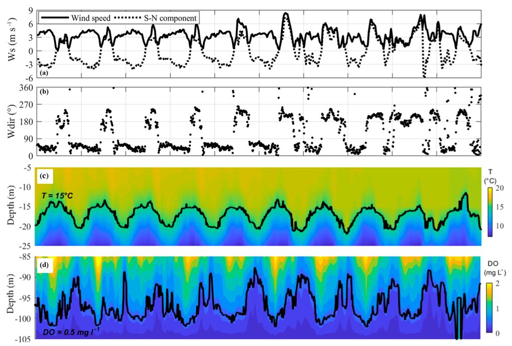
Figure 15: Observations made from the 14^th to the 24^th of October 2017 in Lake Iseo. a) wind speed and its southernly component. b) wind direction. c) temperature variation. d) dissolved oxygen (DO) (Valerio et al., 2019).

The role that winds play in the depth of the OAI can be explained based on Ekman transport in large bodies of water. Ekman transport occurs for surface waters up to a depth of approximately 100 m which applies to most lakes (Toffolon, 2013). The fundamental principle is that the net movement of water will be orthogonal to the direction the wind blows. It will be to the right in the northern hemisphere and to the left in the southern hemisphere due to Coriolis (Emery & Csanady, 1973). This is caused by the friction and drag between layers of water. The layer closer to the surface will be directed by the wind and subsequent layers are dragged towards that direction (Emery & Csanady, 1973). This results in the Ekman spiral which is shown in figure 16. For this reason, an upwelling is observed. If all the surface water in a body is pulled in a direction, the deep cold anoxic waters will move upwards to fill the void as was observed in the case study in Lake Iseo (Emery & Csanady, 1973; Valerio et al., 2019). Consequently, the oxycline oscillates from those movements of water, and the magnetotactic bacteria must follow suit.

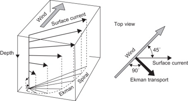
Figure 16: Representation of Ekman transport in the Northern hemisphere (Cushman-Roisin & Beckers, 2011).

Double Diffusive Convection. Secondly, double-diffusive convection, also known as “salt fingers”, causes fluctuations in the depth of the OAI. This event was captured in a case study of the oxycline in the Baltic Sea (Weidner et al., 2020). They reported the merging, splitting, appearance, and disappearance of multiple layers of water. Double diffusive convection mixing occurs within the water column when cold fresher water lies on top of denser saltier water. This is caused by the interactions of two fluids with different diffusing rates (Weidner et al., 2020). The thermal diffusivity exceeds the diffusivity of salt in water as their values are respectfully K_T = 1.4 ∙ 10^-7 m²/s, and K_S = 1.1 ∙ 10^-9 m²/s (Radko, 2013). By the laws of Nature, such mixing does not occur without energy. Indeed, the energy is released by the component with slower diffusing. As vertical mixing occurs because of the instability in density components, the center of gravity of a water parcel will lower because of the salinity. Potential energy is released, and movement occurs (Radko, 2013). For further understanding, consider just one parcel of water that moves away from its initial position, the temperature of this parcel will adjust itself to the ambient temperature while the salinity will mostly be retained. This results in a parcel of water that is still denser than the surroundings due to the different salt gradients. It will keep moving away from equilibrium using the potential of the density gradient. In the ocean, the scale of this movement is limited to a few centimeters by effective molecular conduction (Radko, 2013). While this does not seem significant to humans, variations of a few centimeters have greater impacts on organisms, such as magnetotactic bacteria, sized between 50 and 100 micrometers, when trying to find their ideal biotopes (Lefèvre & Bazylinski, 2013).

Conclusion

In summary, scientists and researchers have spent decades on the understanding of magnetotactic bacteria (MTB) and what tools they have developed to survive in their highly motile environment. Firstly, this unique group of aquatic microorganisms can precisely navigate using the Earth’s magnetic field through magnetotaxis. The bacteria designed magnetosomes that align with the Earth’s magnetic field. This allows MTB to find and remain in their rapidly fluctuating biotope. The second tool, that these organisms have developed to navigate their three-dimensional environment is photo response. UV rays are highly damageable for MTB cells, thus these prokaryotes swim away from radiating light, a phenomenon called phototaxis. Unfortunately, MTB do not thrive in all oxygen concentrations. They can be either microaerophiles or anaerobes that metabolize in low oxygen conditions. Therefore, they have developed magneto-aerotaxis. Another way to reduce their three-dimensional search for their ideal habitat into a one-dimensional search is through the alignment of their magnetosome chain. Aligning one’s magnetosome to the magnetic field lines provides further position stabilization, which counters Brownian motion. Additionally, the fact that the alignment occurs passively, without much use of the bacteria’s metabolic energy, describes that this design is energy efficient. Together, the four tools mentioned above allow MTB to navigate to desired locations by minimizing the distance they need to travel. And to move towards these desired locations, MTB have developed additional sophisticated flagella. In essence, the way that nature has designed the oxic-anoxic interface induces evolutionary needs for adaptations in the magnetotactic prokaryotic species. Comparatively, it comes as no surprise that humans have not developed an internal navigation method as efficient as the bacteria’s compass, since their biotope is principally in two dimensions. It would be interesting to perform subsequent research on how other organisms living in biotopes with three dimensions orient themselves. What do their own internal compasses look like?

References

1 – Fundamentals. (2002). In C. J. Nappo (Ed.), International Geophysics (Vol. 85, pp. 1-24). Academic Press. https://doi.org/https://doi.org/10.1016/S0074-6142(02)80269-8

Bente, K., Mohammadinejad, S., Charsooghi, M. A., Bachmann, F., Codutti, A., Lefèvre, C. T., Klumpp, S., & Faivre, D. (2020). High-speed motility originates from cooperatively pushing and pulling flagella bundles in bilophotrichous bacteria. eLife, 9, e47551. https://doi.org/10.7554/eLife.47551

Britannica, T. Editors of Encyclopaedia (2011, June 20). Zeeman effect. Encyclopedia

Britannica. https://www.britannica.com/science/Zeeman-effect

Brune, A., Frenzel, P., & Cypionka, H. (2000). Life at the oxic-anoxic interface: microbial activities and adaptations. FEMS Microbiol Rev, 24(5), 691-710. https://doi.org/10.1111/j.1574-6976.2000.tb00567.x

Cushman-Roisin, B., & Beckers, J.-M. (2011). Chapter 8 – The Ekman Layer. In B. Cushman-Roisin & J.-M. Beckers (Eds.), International Geophysics (Vol. 101, pp. 239-270). Academic Press. https://doi.org/https://doi.org/10.1016/B978-0-12-088759-0.00008-0

Dasdag, S. (2014). Magnetotactic Bacteria and their Application in Medicine. Journal of Physical Chemistry & Biophysics, 2. https://doi.org/10.4172/2161-0398.1000141

Dey, R. What is Phototaxis? What is Positive and Negative Phototaxis? Explained in Detail. Retrieved september 30 from https://onlyzoology.com/what-is-phototaxis-what-is-positive-and-negative-phototaxis/#google_vignette

Emery, K. O., & Csanady, G. T. (1973). Surface Circulation of Lakes and Nearly Land-Locked Seas. Proceedings of the National Academy of Sciences, 70(1), 93-97. https://doi.org/doi:10.1073/pnas.70.1.93

Fernanda, A., & Daniel, A.-A. (2018). Biology and Physics of Magnetotactic Bacteria. In B. Miroslav, S. Mona, & E. Abdelaziz (Eds.), Microorganisms (pp. Ch. 1). IntechOpen. https://doi.org/10.5772/intechopen.79965

Fradin, C. (2013). Magnetotactic Bacteria. Retrieved September 29 from https://physics.mcmaster.ca/~biophys/molbiophys/bacteria.html#:~:text=The%20term%20%22magnetotactic%20bacteria%22%20regroup%20a%20number%20of,magnetic%20field%2C%20just%20as%20a%20compass%20needle%20goes.

Frankel, R. B., & Bazylinski, D. A. (2006). How magnetotactic bacteria make magnetosomes queue up. Trends Microbiol, 14(8), 329-331. https://doi.org/10.1016/j.tim.2006.06.004

Greenberg, M., Canter, K., Mahler, I., & Tornheim, A. (2005). Observation of magnetoreceptive behavior in a multicellular magnetotactic prokaryote in higher than geomagnetic fields. Biophysical journal, 88(2), 1496-1499. https://doi.org/10.1529/biophysj.104.047068

J. Hall, M. (2023). What Is a Squid Magnetometer? Retrieved 30 September 2023, from https://www.allthescience.org/what-is-a-squid-magnetometer.htm?expand_article=1

Kalmijn, A. (1981). Biophysics of geomagnetic field detection. IEEE Transactions on Magnetics, 17(1), 1113-1124. https://doi.org/10.1109/TMAG.1981.1061156

Kiani, B., Faivre, D., & Klumpp, S. (2015). Elastic properties of magnetosome chains. New Journal of Physics, 17(4), 043007. https://doi.org/10.1088/1367-2630/17/4/043007

Kiani, B., Faivre, D., & Klumpp, S. (2018). Self-organization and stability of magnetosome chains—A simulation study. PLoS One, 13(1), e0190265. https://doi.org/10.1371/journal.pone.0190265

Klumpp, S., Lefèvre, C. T., Bennet, M., & Faivre, D. (2019). Swimming with magnets: From biological organisms to synthetic devices [Review]. Physics Reports, 789, 1-54. https://doi.org/10.1016/j.physrep.2018.10.007

Körnig, A., Dong, J., Bennet, M., Widdrat, M., Andert, J., Müller, F. D., Schüler, D., Klumpp, S., & Faivre, D. (2014). Probing the Mechanical Properties of Magnetosome Chains in Living Magnetotactic Bacteria. Nano Letters, 14(8), 4653-4659. https://doi.org/10.1021/nl5017267

Lefèvre, C. T., & Bazylinski, D. A. (2013). Ecology, Diversity, and Evolution of Magnetotactic Bacteria. Microbiology and Molecular Biology Reviews, 77(3), 497-526. https://doi.org/doi:10.1128/mmbr.00021-13

Madan, I., Vanacore, G. M., Pomarico, E., Berruto, G., Lamb, R. J., McGrouther, D., Lummen, T. T. A., Latychevskaia, T., García de Abajo, F. J., & Carbone, F. (2019). Holographic imaging of electromagnetic fields via electron-light quantum interference. Science Advances, 5(5), eaav8358. https://doi.org/doi:10.1126/sciadv.aav8358

Magnetotactic Bacteria. (2023). In encyclopedia.com.

Mann, S., Sparks, N. H. C., & Board, R. G. (1990). Magnetotactic Bacteria: Microbiology, Biomineralization, Palaeomagnetism and Biotechnology. In A. H. Rose & D. W. Tempest (Eds.), Advances in Microbial Physiology (Vol. 31, pp. 125-181). Academic Press. https://doi.org/https://doi.org/10.1016/S0065-2911(08)60121-6

Palagi, S., Walker, D., Qiu, T., & Fischer, P. (2017). Chapter 8 – Micro- and nanorobots in Newtonian and biological viscoelastic fluids. In M. Kim, A. A. Julius, & U. K. Cheang (Eds.), Microbiorobotics (Second Edition) (pp. 133-162). Elsevier. https://doi.org/https://doi.org/10.1016/B978-0-32-342993-1.00015-X

Perduca, M. (2016). Learning from magnetotactic bacteria: production of biomimetic magnetites and their potential use in clinics. Retrieved september 30 from https://www.dbt.univr.it/?ent=seminario&id=3823&lang=en

Philippe, N., & Wu, L. F. (2010). An MCP-like protein interacts with the MamK cytoskeleton and is involved in magnetotaxis in Magnetospirillum magneticum AMB-1. J Mol Biol, 400(3), 309-322. https://doi.org/10.1016/j.jmb.2010.05.011

Philipse, A. P., & Maas, D. (2002). Magnetic Colloids from Magnetotactic Bacteria:  Chain Formation and Colloidal Stability. Langmuir, 18(25), 9977-9984. https://doi.org/10.1021/la0205811

Radko, T. (2013). Double-Diffusive Convection. Cambridge University Press. https://doi.org/DOI: 10.1017/CBO9781139034173

Satyanarayana, S., Padmaprahlada, S., Chitradurga, R., & Bhattacharya, S. (2021). Orientational dynamics of magnetotactic bacteria in Earth’s magnetic field-a simulation study. J Biol Phys, 47(1), 79-93. https://doi.org/10.1007/s10867-021-09566-9

Scheffel, A., Gruska, M., Faivre, D., Linaroudis, A., Plitzko, J. M., & Schüler, D. (2006). An acidic protein aligns magnetosomes along a filamentous structure in magnetotactic bacteria. Nature, 440(7080), 110-114. https://doi.org/10.1038/nature04382

Sherman, F., Imberger, J., & Corcos, G. (2003). Turbulence and Mixing in Stably Stratified Waters. Annu Rev Fluid Mech, 10, 267-288. https://doi.org/10.1146/annurev.fl.10.010178.001411

Smith, M. J., Sheehan, P. E., Perry, L. L., O’Connor, K., Csonka, L. N., Applegate, B. M., & Whitman, L. J. (2006). Quantifying the magnetic advantage in magnetotaxis. Biophys J, 91(3), 1098-1107. https://doi.org/10.1529/biophysj.106.085167

Toffolon, M. (2013). Ekman circulation and downwelling in narrow lakes. Advances in Water Resources, 53, 76-86. https://doi.org/https://doi.org/10.1016/j.advwatres.2012.10.003

Valerio, G., Pilotti, M., Lau, M. P., & Hupfer, M. (2019). Oxycline oscillations induced by internal waves in deep Lake Iseo. Hydrol. Earth Syst. Sci., 23(3), 1763-1777. https://doi.org/10.5194/hess-23-1763-2019

Weidner, E., Stranne, C., Sundberg, J. H., Weber, T. C., Mayer, L., & Jakobsson, M. (2020). Tracking the spatiotemporal variability of the oxic–anoxic interface in the Baltic Sea with broadband acoustics. ICES Journal of Marine Science, 77(7-8), 2814-2824. https://doi.org/10.1093/icesjms/fsaa153

Zhang, W. J., & Wu, L. F. (2020). Flagella and Swimming Behavior of Marine Magnetotactic Bacteria. Biomolecules, 10(3). https://doi.org/10.3390/biom10030460 Zhu, X., Ge, X., Li, N., Wu, L.-F., Luo, C., Ouyang, Q., Tu, Y., & Chen, G. (2014). Angle sensing in magnetotaxis of Magnetospirillum magneticum AMB-1 [10.1039/C3IB40259B]. Integrative Biology, 6(7), 706-713. https://doi.org/10.1039/C3IB40259B