


Abstract
In the face of tumultuous waters and other such environmental challenges, foraminifera have evolved a wide range of morphological adaptions. Indeed, the development of tests, pores, pseudopodia, and spines have allowed them to thrive within a variety of marine ecosystems, globally, for over 545 million years. Their fossils have historically been used as a tool in paleontology to study ancient environments, and in more modern times, their morphological adaptations have come to be appreciated from a bioengineering perspective. This paper discusses the environmental pressures to which foraminifera are subjected to and presents their evolutionary responses.
Introduction
Foraminifera are an order in the kingdom of protists, but due to their unique shells, they have been colloquially (and incorrectly) termed “armored amoeba” (Foraminifera). Foraminifera live in large bodies of water worldwide, from estuaries to the deep ocean, and have developed numerous interesting morphological adaptations that allow them to thrive in these diverse environments, leading to an appreciable diversity within the foraminifera order. Foraminifera can range from less than a millimeter long to up to 15 cm (Saraswati, 2021), and they are considered a part of a microbiome with many species forming symbiotic relationships with bacteria or algae.
Despite being a single cell, foraminiferal morphology can be very complex (refer to Fig. 1). They form intricate tests around their endoplasm (which contains the main cellular machinery), effectively shielding their most vulnerable parts from the external world (Saraswati, 2021). In addition to the endoplasm is the ectoplasm that surrounds the test; this ectoplasm has protrusions called pseudopodia that can join and split dynamically. The pseudopodia allow foraminifera to interact with their environment, and if a foraminifer is disturbed it can retract the pseudopodia back into the test.
Benthic versus Planktonic Foraminifera
Foraminifera can be divided up into two groups based on their life cycle: benthic and planktonic (Saraswati (2021)). Benthic foraminifera are those that spend the majority of their lives on or in the ocean floor, while planktonic foraminifera (who evolved from benthic foraminifera) are those that live suspended in the water. Benthic and planktonic foraminifera encounter different environmental pressures and thus exhibit different morphologies. Benthic foraminifera tend to have complicated internal tests (shells), while planktonic foraminifera tend to develop spines and porous tests as a means of decreasing their settling velocity. Both benthic and planktonic foraminifera can form symbiotic relationships with photo-symbionts, however in those cases, both groups find themselves limited to areas with appropriate light availability (Saraswati (2021).
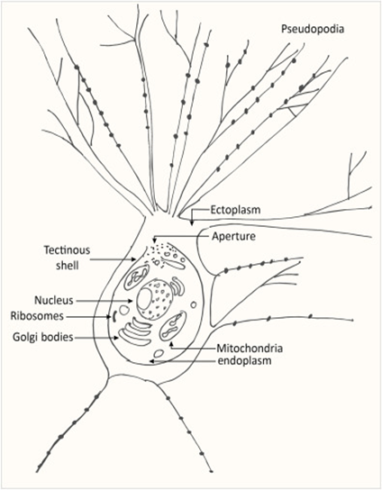
Fig. 1. The protoplasm includes the “soft parts” of the foraminifera, namely the endoplasm and ectoplasm. Here it is shown that the endoplasm and ectoplasm are connected by an aperture, which allows for the exchange of materials (both organic and inorganic). The ectoplasm’s pseudopodia are also shown, with black dots representing the mitochondria inside the pseudopodia (Saraswati, 2021)

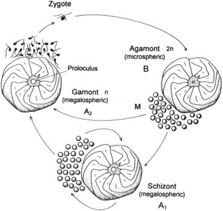
Fig. 2. Life Cycle of Foraminifera (BouDagher-Fadel, 2015). The alternation between the gamont (gamete-producing) and agamont (asexual) generations are shown. Additionally, note that certain species of foraminifera have been observed to reproduce asexually for several cycles, with those individuals termed “schizont” and having the same morphology as the megalospheric generation.
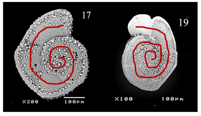
Fig. 3. Megalospheric vs Microspheric Tests of Nummulites maximus (Saraswati, 2021). On the right is a fossilized microspheric test, which is much larger than the two megalospheric tests on the left.
The life cycle of multichambered foraminifera is characterized by an alternation between a gamete-producing generation and an asexual generation (see Fig.2) (Paleoclimate Foraminifera), and there may exist exceptions to this observation. The haploid generation (produced asexually) and the diploid generation (produced sexually) can be differentiated from each other based on the size of their initial chambers, called a “proloculus”. The haploid generation tends to have larger proloculi, and so they are called megalospheric, while the diploid generation’s proloculi are smaller and called microspheric. The complete test of the microspheric generation tends to be larger than that of the megalospheric generation, as seen in Fig.3.
The reproductive strategies employed by foraminifera are species specific, and it appears that asexual reproduction is not as common in planktonic foraminifera as it is in benthic foraminifera (Weinkauf et al. (2022)). The question of whether planktonic foraminifera assemblages can be maintained based on sexual reproduction alone has not yet been answered, but it does seem that asexual reproduction would be a useful strategy to employ in low-density populations that are subjected to the hydrodynamic turbulence of the open ocean. As will be seen in the discussion of temperature, the reproductive strategies of foraminifera may present unseen consequences.
The Optics of Tests
One characteristic that distinguishes Foraminifera from other protists is their shell, or test, which physically separates them from their environment (Hansen, 1999). Of the 15 taxa, 11 of them build their tests out of calcium carbonate, and in lamellar shells this leads to interesting optical properties that can be detected using a polarizing microscope.
Lamellar shells are made up of calcite or aragonite, where calcite creates trigonal crystal systems and aragonite creates orthorhombic crystal systems that appear fibrous (Madhu, 2019). They both have high birefringence of 0.156 and 0.172 (for calcite and aragonite, respectively) (Hall, 1978). This birefringence means that the refractive index of the tests depends on the polarization and direction of light propagation. The orientation of the crystals in lamellar tests can be either radial or granular, and it was hoped that this characteristic would be useful in taxonomy (Berggren & Loeblich, 1965), however there are a few problems. The first is that there are limitations to using polarizing microscopes, which provide clarity up to but not beyond the micrometer scale (Polarized Light Microscopy). This means that other microstructures, such as pores, can introduce errors in the interpretation of observed interference patterns; for example, narrow pores in thin sections of tests have the appearance of radial crystal structure (Hansen, 1999). Another more relevant issue is that the optical character of tests cannot provide taxonomic information above the species level, since radial and granular orientations can be found in the same genus (Hansen, 1999). This means that measuring crystal orientation can only be used to reject or support, but not confirm, the proposed species classification of a given sample.
Foraminifera as Biological Indicators
The hydrodynamics of a coastal environment creates a bias in the paleontological record, with more intense hydrodynamics preventing the deposition of fine sediment and foraminifera (Bérgamo et al., 2022). From these observations, it can be said that a concentrated deposit of fragile foraminifera is a strong indication of calmer hydrodynamics. In this way, foraminifera deposits are used as a paleontological tool in studying coastal environments.
Foraminifera can also be used to assess environmental damage from pollutants, such as those from oil spills, agricultural waste, paper mill effluents, and baseline human activity (Armynot du Châtelet & Debenay, 2010). One study from 1969 found that foraminiferal samples collected from an estuary downstream of a fish farm and slaughterhouse contained foraminifera that were much larger than average (Muller & Lee, 1969). The researchers attributed this change to the increased availability of organic matter.
Environment
Foraminiferal survival as a function of physical factors such as temperature, salinity, light, and density are, for the most part, flexibly defined; while in vivo studies can show that there do exist strong correlations, observations of foraminiferal assemblages in their natural environment suggest that most species are able to tolerate variation in their physical environment. Oftentimes, this variation correlates to decreased functionality, such as inhibited food acceptance, decreased growth, and unsuccessful reproduction (Arnold & Parker, 1999). Of all the physical factors, the greatest controlling factor appears to be temperature, but even this is still a species-specific tolerance.
Water Temperature and Salinity
The observation that most planktonic foraminiferal assemblage patterns are latitudinally distributed has inspired many studies on foraminiferal responses to temperature variation (McCoy & Connor, 1980). The primary source of heat in the ocean is from solar radiation, and water is very good at absorbing this radiation, with most of the absorption taking place in the top 10m from the surface as noted in “Chapter 2 – Temperature in the oceans” (1995). Vertical mixing that is driven by wind, waves, and currents can distribute this heat as deep as 200-300m to create what is referred to as the epipelagic zone. At mid-latitudes, it is in this layer that the “seasonal” thermocline is found; during the winter, the thermocline is pushed further down, and the steepness of the thermal gradient reduces, but in the summer the thermocline raises again and the steepness increases (see Fig. 4(d)). In low latitudes, there is less of a seasonal effect on the thermocline, and at polar latitudes there is no permanent thermocline, but there can be a seasonal one in the summer (see Fig.4(a-c)). Beyond the epipelagic layer is the mesopelagic layer, which extends to 1000 m and at mid and low latitudes this is where the “permanent” thermocline is found (see Fig. 5). There is no permanent thermocline at the poles, but in the summer there can be a seasonal thermocline. In some places there can be a diurnal thermocline, but typically the temperature variation isn’t more than 1-2 degrees Celsius and occurs only within 10-15m of the surface.
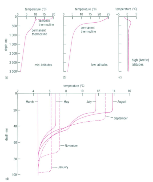
Fig 4. Thermocline at Mid (a), Low (b), and High (c) Latitudes. Note the similarity between the seasonal thermocline at mid-latitudes in (a) to the permanent thermocline at low latitudes in (b): they are both very steep in the epipelagic zone. In (c) we see a very small thermocline at the epipelagic zone. (d) is Seasonal Thermocline in the Northern Hemisphere. There is large variation of the thermocline throughout the year in the upper 100m. Adapted from “Chapter 2 – Temperature in the oceans” (1995).

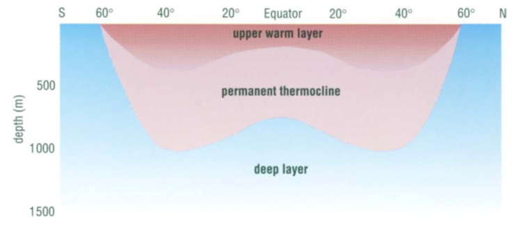
Fig. 5. Cross section of the Global Thermocline as a Function of Latitude. Note how the permanent thermocline is beneath the seasonal thermocline (labeled “upper warmer layer”), and that there is no permanent thermocline at the poles. From “Chapter 2 – Temperature in the oceans” (1995).
In the polar regions, an effect called thermohaline circulation is responsible for the deeper currents that propagate throughout the rest of the ocean, known as the global conveyor belt (Thermohaline Circulation). When sea ice forms in the polar regions, the salt concentration in the remaining liquid water increases, and increased salinity promotes a downward vertical circulation due to increased density.

Fig 6. Coiling Directions in G.truncatulinoides (Late Quaternary Investigation of Planktonic Foraminiferal Assemblages from the Western Mediterranean). Dextral coiling is shown on the left and sinistral coiling is shown on the right.
The effect of temperature on foraminifera will be explored in more depth in the proceeding Chemistry paper, since there is a strong correlation between temperature and metabolism. However, temperature has interesting indirect effects on foraminiferal morphology, one example being its impact on coiling direction dominance in species with spiral morphology. Though many hypotheses have been posited, a study on Globorotalia truncatulinoides conducted by Lohmann and Schweitzer (1990) found evidence to support the idea that reproductive strategy – rather than genetic/metabolic signals/pathways – is to blame. In the G.truncatulinoides’ life cycle, individuals descend along the thermocline in the juvenile phase of their life, and then ascend in the late winter, returning to the surface for another reproductive cycle. Their spiral morphology can be either sinistral (left-handed) or dextral (right-handed) (see Fig. 6), and these coiling directions are strongly correlated to when in the season they descend. Sinistral individuals descend earlier than their dextral counterparts and are thus more likely to descend deeper, since the thermocline is shifting towards the surface during this time. The result is that sinistral individuals may find themselves below the depth at which seasonal overturn can return them to the surface, thus the dextral G. truncatulinoides appear as the dominant morphology.
Foraminiferal diversity in the deep ocean (where temperature is typically uniform) is comparable to that at the surface despite the stark difference in temperature, which means that lower temperatures do not limit foraminiferal functionality.
Investigations into the impact of salinity have found that planktonic foraminifera cultured in a lab are able to tolerate salinity variations that exceed natural oceanic variations, suggesting that salinity’s direct impact on foraminifera is minimal (Bijma et al., 1990). For reference, the lowest salinity in which foraminifera have been captured is approximately 30 % (M, 2009). Similarly, the indirect impact of salinity (via water density) is also minimal, as will be discussed shortly. However, this does not mean that salinity should be ignored altogether, as it has a strong influence on foraminiferal distribution in marginal marine species (Gupta, 1999b). There is characteristic species diversity of foraminifera in the different types of marshes, and thus foraminiferal deposits have been used to assess salinity in paleontological studies (Gupta, 1999b). For example, factors such as ground elevation can impact salinity differently at lower-marshes versus higher-marshes, because lower-marshes are more at risk of tidal-flooding, which maintains salinity at a level similar to the ocean (Gupta, 1999a).
Water Density
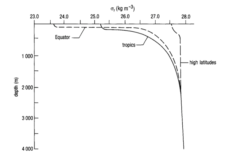
Fig. 7. Generic Oceanic Pycnocline (“Chapter 2 – Temperature in the oceans,” 1995). Note how there is a greater pycnocline at the equator than at the tropics. This is due to greater temperature variation as a function of depth. Also note the convergence of the three lines at large depths: this indicates that there is very little variation in the pycnocline in the deep ocean, again, due to minimal temperature variation.
The density of water is determined by temperature and salinity; density increases as temperature decreases and salinity increases (“Chapter 4 – Density and pressure in the oceans,” 1995). Variation in density forms a pycnocline, which is due primarily to temperature variation rather than salinity variation, since temperature can range from 0-25 deg Celsius while salinity rarely varies beyond 34-36 parts per thousand. It is for this reason that in the deep ocean, the main pycnocline can coincide with the permanent thermocline (Webb, 2019a) (see Fig. 7).
At depths greater than 500-1000 m (i.e. beyond the mesopelagic layer), temperature and salinity do not vary much, and so density does not vary much either, as shown in “Chapter 4 – Density and pressure in the oceans” (1995). Above 500 m, however, we see that the shape of the pycnocline depends on the latitude, with steeper pycnoclines at the equator than at the polar regions (refer to Fig. 7). The depth of the pycnoclines is also shallower for equatorial regions vs lateral and polar regions, again largely due to the thermocline.
Water in a pycnocline is, by definition, stable, since the density gradient is under the force of gravity (“Chapter 4 – Density and pressure in the oceans” (1995). This means that it takes energy to force vertical mixing. The main pycnocline tends to form below the surface currents; the mixing that results from the turbidity of these surface currents is what allows for the creation of a stable pycnocline, as there is appropriate distribution of water based on density. Having a very stable pycnocline discourages vertical mixing within that pycnocline, and seasonal changes can decrease that stability. Some foraminifera take advantage of pycnocline instability, as it is an effective means of long-distance vertical migration (Hohenegger 2004).
Turbulence
As depth increases, so does density, but within the pycnocline there may exist discrete microstructures rather than a stable density gradient (“Chapter 4 – Density and pressure in the oceans” (1995). These microstructures are homogeneous layers of water that are separated by steep changes in salinity and temperature. Layers can be 20-30 m thick and have a lateral distance on the scale of kilometers, or it can be only 20-30 cm thick and have a lateral distance of a few hundred meters. Moving down the layers may show an increase or a decrease in temperature, but density always continues to increase. These homogeneous layers can result in internal waves due to shear velocity that causes turbulence and mixing (see Fig. 8.).
Fig. 8. Turbulence that Results from an Internal Wave (“Chapter 4 – Density and pressure in the oceans,” 1995). Note how turbulence leads to the creation of more layers, which further stabilizes the pycnocline.
Turbulence in the ocean is the result of many different processes, as discussed in “Chapter 4 – Density and pressure in the oceans” (1995). At the surface (about 10 m deep), turbulence is the result of wind-driven waves and currents. In addition to that are tidal-driven currents, which are always present and independent of local weather. Coastal irregularities like estuaries and bays may also introduce turbulence, but even simply raising the seabed shelf will cause turbulence. What is most notable about these processes is that horizontal turbulence is much more common than vertical turbulence, in large part due to vertical gravitational stability. In other words, the pycnocline has a stabilizing effect – at least on vertical turbulence.
Motion behaviors: Foraminifera as Bioturbators
While foraminifera are certainly susceptible to environmental parameters, hence their importance as bioindicators, the study of the motion behaviors of the intertidal foraminifera Haynesina germanica by Deldicq et al. (2023) also highlights their contributions to their environment. Indeed, the latter’s characteristic vertical motion, as it pierces through sediments to create a one-ended vertical tube, contributes to bioturbation. The reworking/mixing of sediments occurs because of the observed trail following behavior of H. germanica: it is suggested in the study that individuals preferred to reuse tubes as a way to reduce the cost of locomotion. This process of “gallery diffusion” adds to the exchange of water & dissolved sediments at the sediment-water interface, and therefore contributes to the bioirrigation of intertidal sediments.
Furthermore, the intensity of the bioturbation appears to be dependent on the density of foraminifera, for it is suggested that H. germanica adapts its motion behavior to deal with competition from other individuals of the species for space & food, which occurs as foraminiferal density increases (Deldicq et al., 2023).
Morphology: Adaptations to its Environment
Interlocular Spaces

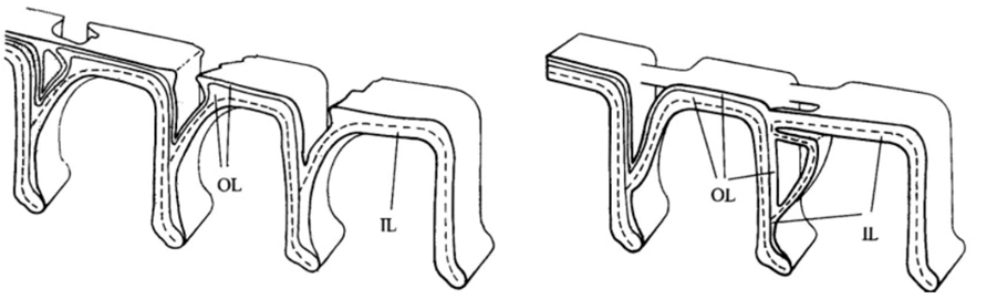
Fig. 9. Bridging Interlocular Spaces (Hansen, 1999). On the left is the structural design seen in Pseudorotalia, and on the right is that of Elphidium. Note how the secondary lamellar surface compares between the two: in Pseudorotalia, it is only the secondary lamellar surface that forms the protrusion, while in Elphidium the entire wall morphs.
Hansen (1999) described “interlocular spaces” as cavities between adjacent chambers that can introduce fragility into the shell, with newly formed chambers at risk of being detached. Some genera of foraminifera have developed ways of preventing this. The Pseudorotalia and Elphidium genera build pillars that bridge the interlocular spaces, but with different points of origin (see Fig. 9). For the genus Pseudorotalia, it is the secondary (outer calcareous) lamellar surface that builds protrusions in the anterior and posterior direction in such a way that protrusions meet and form a bridge. The inner calcareous lining remains unchanged. The formation of these protrusions is performed by 2-3 adjacent chambers. In the genus Elphidium, when a new chamber is added, the entire wall (including the inner calcareous lining) forms a protrusion, called a ponticulus, which extends towards the preceding chamber to form a strong anchor. This is sufficient to prevent mechanical damage even when the interlocular space is large and deep.
Light Variation in the Ocean
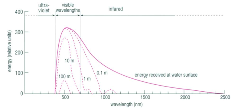
Fig. 10. Light Absorption in the Ocean as a Function of Wavelength (“Chapter 2 – Temperature in the oceans,” 1995). At each line, the depth at which that light is absorbed is written. The graph plots the energy of the light as a function of wavelength.
Most, but not all, of the light that reaches the ocean is in the visible spectrum (400 – 700 nm), and the efficiency by which water absorbs light depends on the wavelength (Webb, 2019b) (see Fig. 10). Longer wavelength light, such as red, orange, and yellow tones, have less energy and are absorbed in the upper 10 m, 40 m, and 100 m respectively, while shorter wavelength light (such as blue and green) may penetrate water down to 200 m. Light that has a much shorter wavelength, such as infrared light, or a much larger wavelength, such as ultraviolet light, is found at (relatively) lower intensities simply because most of that light is already absorbed, scattered and/or reflected by the atmosphere before it reaches the ocean.
Particles in the ocean, such as phytoplankton and zooplankton absorb light which decreases the amount of light that penetrates beyond (Webb, 2019b). Photosynthetic particles, such as phytoplankton, absorb red and blue light but not green light, which gives water a green appearance. This is especially evident in coastal environments, where the concentration of phytoplankton tends to be higher than that in the rest of the ocean. Throughout the ocean, the water molecules themselves scatter blue light, giving the ocean its blue appearance from underwater.
Light variation in the ocean is fairly simple, since it is a function of depth and does not vary with temperature, salinity, or density (Webb, 2019b). The ocean can be divided into layers based on light: the eutrophic zone (equivalent to the epipelagic zone), the dysphotic zone (equivalent to the mesopelagic zone), and the aphotic zone. The eutrophic zone receives enough light to support photosynthesis, while the dysphotic zone receives just enough light to support minimal photosynthesis. The aphotic zone does not receive enough light to support photosynthesis, thus discouraging photosymbiotic relationships in the deep ocean.
Foraminifera engage in symbiotic relationships with photosynthetic microorganisms such as zooxanthellae and diatoms to thrive in marine environments (Klemme et al., 2022). The energy derived from photosynthesis not only supports the foraminifera’s metabolic needs but also plays a crucial role in the precipitation of calcium carbonate for shell formation, as explained by Orsi et al. (2020). The photosynthetic activity of symbionts generates metabolic byproducts, including bicarbonate ions (HCO3–), which contribute to the availability of carbonate ions (CO32-) needed for calcium carbonate deposition (Takagi et al., 2019).
As mentioned earlier, light penetration in water depends on wavelength (“Chapter 2 – Temperature in the oceans,” 1995) and water clarity (Webb, 2019b). Reduced light levels, as occurs with increased depth or turbidity—according to Jacob et al. (2017) — hinders photosynthesis in foraminiferal symbionts. This leads to decreased production of organic compounds and bicarbonate ions, limiting calcium carbonate shell formation. Extended low-light exposure may result in thinner, fragile, or less calcified shells, or even shell dissolution.
Foraminifera exhibit remarkable adaptations to diverse light environments, highlighting their ecological significance. Hohenegger (2004) explains that depth-related adaptations include vertical migration, with foraminifera moving to shallow depths during the day for abundant photosynthesis and deeper at night to evade predators and UV radiation. Diurnal behavior patterns involve positioning within the water column to maximize daytime light exposure, and conserving energy by seeking lower light levels or sediment refuge at night. Pigmentation shields photosynthetic symbionts from intense sunlight, and symbiont diversity ensures adaptation to various light conditions. For example, amphistegina gibbosa is a foraminiferal species known for its adaptation to variable light conditions, described by Hohenegger (2004). It has a unique shell structure with chambers that are relatively shallow, which allows it to tolerate both low and high light levels. In lower light conditions, A. gibbosa can position itself to maximize exposure to available light. This species is also known for its ability to tolerate fluctuations in light intensity due to its flexibility in adjusting its symbiont density based on light availability.
Openings — Pores and Apertures
Pores

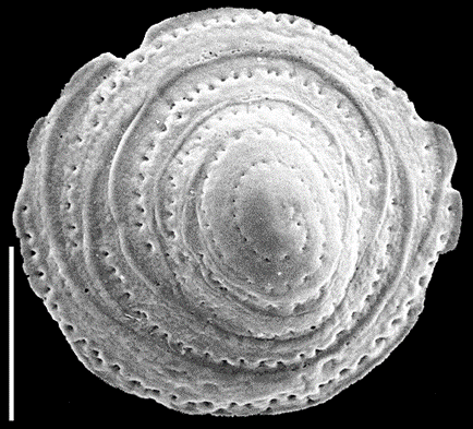
Fig. 11. Micrograph of Patellina (Hansen, 1999). The scale bar corresponds to 100μm. Note the pores visible on the test.
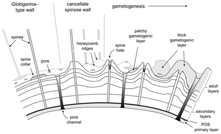
Fig. 12. Cross Sectional Diagram of Typical Foraminifera Canccellate Spinose Wall (Test) (Pearson et al., 2022). Note that the pore channels penetrate the entire span of the test, while the spine holes do not.
Some species of foraminifera have pores, which are holes in the outer wall (or test) of the organisms. The size, type, and arrangement of these pores are used to differentiate different species of foraminifera. See Fig. 11 & 12: in a studied calcareous species (i.e. test is composed of calcium carbonate) Patellina, the pores were found to be responsible for the uptake of organic material into the organism’s interior using tubules also made of organic material (Berthold, 1976). Pores play a role in the sexual reproduction of some species of foraminifera; in one step of these organisms’ life cycles, the megalospheric state of the foraminifera known as a gamont develops secondary pores to release gametes (Goldstein, 1999). Pseudopores are also of note in some species of foraminifera, these are depressions in the test that do not have organic tubules and are physically separated from the interior of the organism (Hansen, 1999). However, it has been found that CO2 particles may still diffuse across the thin wall of the pseudopores of the test into the interior (Hansen & Dalberg, 1979).
Pores and Gas Exchange:
One observation related to pores is that foraminifera species inhabiting low oxygen environments have larger pores and more pore density on the test (Leutenegger & Hansen, 1979). It is hypothesized that an increase in these factors would provide more oxygen to the organism because oxygen would enter the organism through the pores (Bernhard & Gupta, 1999). However, this is disputed as other structural elements of foraminifera seem to have a larger effect on the uptake of oxygen, such as the pseudopodia discussed in the following section (Bernhard & Gupta, 1999). Another gas-exchange mechanism facilitated by foraminifera’s pores is CO2 exchange in a photosymbiosis relationship—which is also discussed in the following section (Leutenegger & Hansen, 1979).
Pores and Buoyancy
In one study, it was shown that the number of pores on foraminifera correlates with the surrounding environment, particularly climate and depth (Allan, 1968). According to Zarkogiannis et al. (2019), the major factor causing differences in porosity is the density of seawater. In water that is warmer and has less salinity (and therefore a lower density), Zarkogiannis et al. showed that foraminifera exhibit more pores. Their hypothesis for this trend is that an increased number of pores increases the buoyancy of foraminifera by decreasing the test’s mass. In a low-density environment, foraminifera could use this increased buoyancy to stay at the surface of the water (Arnold & Parker, 1999), which would be more ideal for its metabolic processes (Zarkogiannis et al., 2019).
Apertures
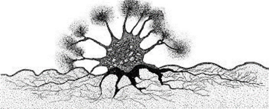
Fig. 13. Astrorhiza limicola Extending Pseudopodia into Sediment and Water Column via Multiple Apertures (Cedhagen, 1988). The water column is in white, and the sediment is in grey. Note the radial display of pseudopodia, made possible by multiple apertures.
Similar to pores, apertures are another differentiating factor between species of foraminifera. Apertures are the primary opening of the interior of foraminifera to the environment and can be observed in various shapes and sizes. These structures’ most prominent role is in the ingestion of nutrients (BouDagher-Fadel, 2015). As seen in Fig. 13, one particular species, Astrorhiza limicola, has multiple apertures positioned such that pseudopodia (extensions of cytoplasm) can extend from the aperture towards sediment to anchor itself and towards the water column to collect nutrients (Cedhagen, 1988). This underlines an important function of apertures, which is to allow pseudopodia to extend into the environment—a topic that is further discussed in later sections. Apertures are also potentially subject to the buoyancy hypothesis discussed for pores, as foraminifera in low water density tropical environments have been shown to have larger apertures (Allan, 1968).
Pseudopodia
Description of Pseudopodia
Along with the development of tests (which are discussed in the following section), the presence of pseudopodia is the defining feature of all foraminifera. Pseudopodia are filaments that extend from the cytoplasm out of the foraminifera’s aperture(s) and form a web-like network to interact with the environment (seeFig. 13), constantly changing the shape of the strands (Goldstein, 1999). Goldstein outlines the functions as: movement, attachment, feeding, building, and structuring tests, protection, respiration, and reproduction. Goldstein also notes that an important property of pseudopodia in foraminifera is the ability for particles to travel along them, which facilitates transport of materials such as sediment, algae, bacteria, and organic material. Another important property of pseudopodia is that organelles are contained within them—such as mitochondria, vacuoles, and phagosomes (Goldstein, 1999).
Pseudopodia and physical material
The ability of pseudopodia to collect sediment and other materials leads to unique behaviors of foraminifera regarding the movement of environmental materials; this ability of pseudopodia drives the process of bioturbation discussed earlier (Groß, 2002). One feeding behavior of foraminifera is called “grazing”, found in some foraminifera in shallow-water environments where there is a surface of algae that the foraminifera can move along (Goldstein, 1999). The pseudopodia of a foraminifera collect algal cells and places them in a mound around its test to feed on (Goldstein, 1999). Digestion of grazed material likely occurs in the pseudopodia as opposed to the cell body (Mojtahid et al., 2011). “Deposit feeding” is similar to grazing in the creation of mounds (or cysts) to feed on. However, deposit feeding is common in benthic foraminifera species living in sediment-rich environments on/in the ocean floor, and is described by Goldstein (1999) as involving “sediment, algal cells, bacteria, and organic detritus” collected by the pseudopodia. According to Goldstein, contents of these cysts are subsequently ingested in large quantities into the cell body of the foraminifera through phagocytosis.
Pseudopodia and mitochondria
According to Bernhard and Gupta (1999), all foraminifera contain mitochondria (also, see Fig. 1). Mitochondria are commonly found in pseudopodia and in cytoplasm of the aperture—to be excreted through the pseudopodia (Bernhard and Alve, 1996). The function of these mitochondria is likely aerobic cellular respiration or to perform the chemical function of a hydrogenosome (Bernhard & Gupta, 1999), which is beyond the scope of this physics paper. However, it is important to note that the number of mitochondria in foraminifera increases in low-oxygen environments, suggesting that they are necessary for survival in these conditions. Having the mitochondria in pseudopods is advantageous since pseudopods can grow to “at least ten times the test diameter” (Travis and Bowser, 1991, as cited in (Bernhard & Gupta, 1999)), which allows mitochondria to access oxygen even if the foraminifera’s body is in an anoxic environment such as sediment.
Tests
The Mechanics of Tests
The physical properties of foraminifera tests have been extensively studied with the intention of creating detailed taxonomic classifications, however, there has been less focus on the actual mechanical properties that are inherently linked to these physical structures. One study, conducted by Bowser and Bernhard (1993), sought to remedy this lack of knowledge. Their study focused on astrammina rara, a benthic foraminifer from the Antarctic, chosen because it was not only abundant (1800 /m2) and easily identifiable (6.5 mm diameter), but because its shell is a single chamber, allowing researchers to remove the full cell-body from the test. The cell-body regrows its test, which allowed researchers to reuse specimens.
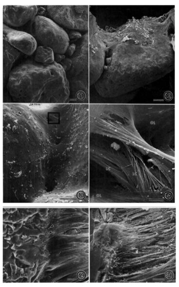
Fig.14. Scanning electron micrographs of a fractured A. rare test. (11) agglutinated test made of interlocking grains, (12) bioadhesive ligaments holding grains together (13) internal lining (14) ligamentous bioadhesive cables merging with internal lining. (19) Enlarged view of junction between bioadhesive ligaments to grains, shown by arrow heads. (20) Sample was treated with SDS with denatured smooth surface of Bioadhesive ligaments, leaving their fibrous tensile cables exposed (Bowser and Bernhard, 1993).
Researchers observed considerable elasticity (the ability of the test fragments to return to their shape after strain is applied), with an estimated yield point of 8.8 x 10⁴ dynes (Bowser and Bernhard, 1993). This value could not be confirmed only because the needles used to apply strain tended to break before the fragmented tests yielded. This mechanical property of A. rara may be explained by three structural characteristics: (1) agglutinated test made of interlocking grains; (2) an external flocculent network that holds grains together and promotes test rigidity; (3) an internal network of ligamentous bioadhesive “cables” which exert tensile forces on the grains (see Fig. 14). These internal cables serve as attachment sites for the cell-body’s pseudopodia, and the geometry of these cables prevents rotation and relative translation of the grains, which gives the tests their elastic character. Additionally, it should be noted that A. rara display grain selectivity that is based on size; the percentage composition of the agglutinated tests were mostly large grains (> 500 µm) regardless of the sediment’s grain-size percentage-composition. The mineralogical composition of the grains appears insignificant as well, as quartz and feldspars were incorporated in no apparent pattern or bias. This implies that it is the interlocking pattern of the grains that contributes to physical stability – rather than the physical properties of an individual grain.
In their conclusion, researchers suggest that the meshwork of exterior flocculent fibrous serves to smoothen the exterior (thereby reducing friction) and prevent bacterial attacks on interior bioadhesive cables.
Tests and Hydrodynamic Conditions
As discussed in Briguglio and Hohenegger (2011), larger benthic foraminifera (LBF) commonly harbor algae endosymbionts, and they inhabit photic zones—the uppermost layer of bodies of water—to provide their symbionts with light. In those shallow waters, LBF are subjected to very strong hydrodynamic conditions, making them susceptible to water motion. The foraminifera cannot let themselves be taken and entrained by the flows, which is why they build themselves shells capable of resisting transportation; they construct their tests such that their shapes are hydrodynamically convenient. Some species can also avoid the effects of water motion by using hiding strategies, or by developing mechanisms that allow the organism to anchor themselves to substrate.
On shape differentiation
Hydrodynamic conditions are defined as the motion of water, such as tides, currents, and waves (“Chapter 4 – Density and pressure in the oceans”, 1995). Under weak hydrodynamic conditions, large surface-to-volume ratio is ideal. Analogously, under strong hydrodynamic conditions — such as in environments in gravel or coarse sand substrates — larger benthic foraminifera will have high-density lenticular tests, shaped like a double convex lens. As mentioned earlier, shape can also be influenced by the light-requirements of the symbiont: in deep waters with very little penetration of light, the tests will have a larger surface to maximize light exposure (Hallock et al., 1991). Conversely, specimens inhabiting shallower waters– with greater light availability–would have smaller surfaces.
Ultimately, while the LBF distribution within a certain environment cannot solely be explained through hydrodynamics, it is most commonly the geometrical and structural parameters of the tests, which vary given their environment, that are used to quantify the foraminifera’s ability to resist water motion.
Spines
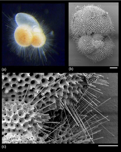
Another mode by which foraminifera adjust to the hydrodynamic behaviors of the liquids in which they are immersed is through the growth of acicular spines, illustrated in Fig. 15, which are long, needle-shaped carbonate extensions that develop on the shell walls of foraminifera (Grigoratou et al., 2021).

Fig. 15. “True spines” (acicular projections) in Trilobactus sacculifer (Pearson et al., 2022). a) image is approx. 1mm, b) 100um, c) 30um
Settling speed is the velocity at which a particle will settle in a still fluid, though in the context of the ocean, it is important to note that for foraminifera, it is not defined as velocity at which they sink. Knowing that buoyant forces strongly influence foraminifera accordingly to its geometrical properties (Jon Furbish & Arnold, 1997), that they act on them depending on their size, shape, and density, we must consider the effects of spines on settling speed. In fact, planktonic foraminifera will adjust their buoyancies to counter that gravitational settling, and while they partly do so by making low-density lipids and/or gases, the growth of acicular spines seem to also be an evolutionary adaptation engineered to counter settling. That being said, researchers note that the growth of spines is responsible for two counteractive effects. In fact, on one hand, the presence of spines implies an increase in weight, and therefore an increase in settling speed; on the other hand, their presence increases fluid drag on the foraminifera, which decreases settling speed. Therefore, if it is hypothesized that spines are indeed an evolutionary strategy meant to reduce settling, then it is expected that the additional drag provided by the spines outweighs the adverse effects associated with an increased weight. The geometrical complexity and variety of foraminiferal shapes are a challenge for researchers who want to model the links between the tests’ forms and involve solving equations for the fluid motions of both drag and settling speed. The experiment from which the following conclusions are derived relies on dimensional analysis when defining values for the coefficient of drag CD and Reynold’s number RE for the models of spinose foraminifera. The Reynolds number of a fluid is the ratio of inertia to viscosity of the fluid; it is a unitless measurement that can tell us the nature of the fluid, either turbulent or laminar (Prichard et al., 2022).
Grigoratou et al. (2021) found that for foraminifera that are geometrically similar and are characterized by the quasi-spherical symmetry of their spinal arrangements, settling happens in an inverse relationship between CD and RE. This means that fluid drag increases as both the spine number, denoted N, and the spine length, denoted L, increase: ergo, even with “modest” values of N and L, there will be a drag sufficiently large enough such that the particular shape of the tests is not significant.
Furthermore, planktonic foraminifera are passive feeders who seek out and interact with prey through an expansion of the cytoplasm from its test, and it is a property which is further supported by the presence of spines: they are a support surface for the pseudopodia, and consequently increase the foraminifera’s encounter rates. As such, the presence or absence of spines have been strongly associated with the organism’s preferred diet, with adult spinose species observed to be mostly carnivorous. Conversely, non-spinose species appear to be mostly herbivorous, though their diets can be supplemented from other resources.
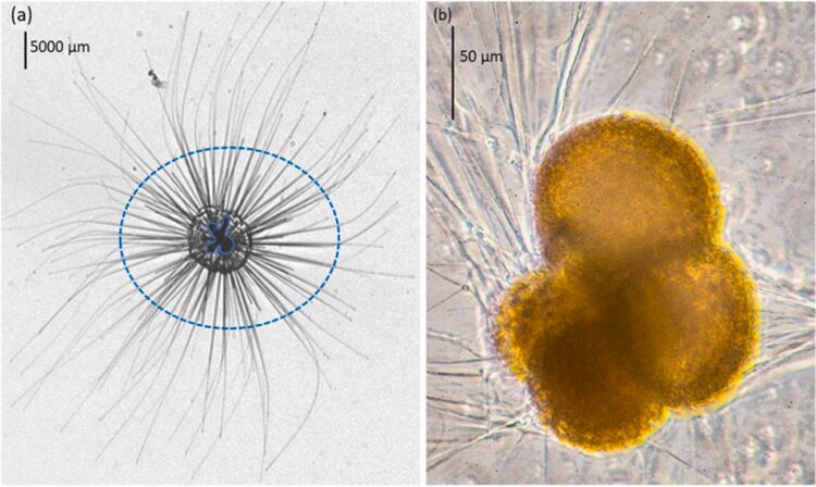
Fig. 16. Spinose and non-spinose planktonic foraminifera species (Grigoratou et al., 2021). On the left, in-situ observation of the spinose species Hastigerina pelagica, where the spines are the darker lines inside the blue, dotted ellipse. Note that the solid blue line in the center identifies the test. On the right, in-vitro observation of the non-spinose species Neogloboquadrina incompta.
Notably, in spinose planktic foraminifera, the test serves as a basis for the spines (Fig. 12), and this supports the pseudopodal network that help them catch their prey, an adaptation that is particularly important given that they are found in shallow waters (Pearson et al., 2022).
Shapes of Spines
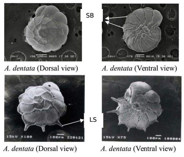
Just as a foraminifera’s test shapes varies according to, namely, the hydrodynamic conditions of its environment, Hussain et al (2017) find that not all spines are identical: notably, the species Ammonia dentata appear to be able change the shape of their spines such that their shape reflects the hydrodynamic conditions of their body of water.

Fig. 17. Morphological differences of spines in Ammonia dentata. The higher two images show A. dentata with short, blunt spines (SB) in dorsal and ventral view, respectively. The lower two images show it with long, slender spines (LS) in dorsal and ventral view. Adapted from S M and Nandamuri (2017).
Indeed, Hussain et al. (2017) found that in shallower waters, characterized by more turbulent conditions—for they are influenced by waves, currents, and tides—the spines are short and blunt, making their tests more robust. They are also less effective in producing drag. Conversely, it is when Ammonia dentata are found in greater water depths—which are synonymous with calmer hydrodynamic conditions—that their spines are engineered to be comparatively long and slender, as a way to adapt themselves to buoyancy. It is important to understand that elongated spines are more susceptible to breakage, considering the torque applied by vicious forces, but they also allow larger planktic foraminifera to increase drag and reduce their setting speed.
Relationships with other organisms
Types of relationships with other organisms
Three types of relationships can be observed in foraminifera: carnivory, parasitism, and symbiosis. Carnivory is exhibited by some species and is facilitated by specially-adapted pseudopodia that are strengthened with an extracellular matrix material (Goldstein, 1999). Goldstein also describes parasitism is exhibited in some species, such as Fissurina marginata which uses pseudopodia to feed on the cytoplasm of a host. Symbiosis is the most complex relationship that foraminifera have with other organisms—specifically, Algae. Hallock (1999) outlines three major benefits of algal symbiosis: “energy from photosynthesis[,] enhancement of calcification[and,] uptake of host metabolites by symbiotic algae”.
Algal symbiosis and photosynthesis
Foraminifera has a large energy advantage from symbiosis because of the algae symbiont’s ability to perform photosynthesis and the host foraminifera’s ability to collect dissolved nutrients/organic matter (Hallock, 1999). This relationship, called photosymbiosis, allows each organism to specialize in what they are good at—feeding and photosynthesis, while having their needs met—such as energy from sugars and nitrogen fixation. This process depends on the CO2 concentration and light availability of the environment for photosynthesis as well as the nutrient availability of the environment, which is “symbiosis is prevalent in tropical [species]” (Hallock, 1999). Since photosynthetic pigments in symbionts are activated by different wavelength of light, and the light is a function of depth in the ocean, foraminifera’s vertical distribution in the ocean can be dependent on light.
Conclusion
Many species of foraminifera exist in turbulent environments and as such have developed tests that can withstand external forces, as seen in Astrammina rara, whose tests’ strength, rigidty, and elasticity comes from the interlocking pattern of grains, the external flocculent network, and the internal ligamentous bioadhesive cables, respectively. Additionally, some species of foraminifera build pillars that span the interlocular spaces (between chambers) to reduce fragility, as seen in the genera Pseudorotalia and Elphidium.
Understanding the intricate relationship between light, photosynthesis, and shell formation in foraminifera is essential for assessing their ecological role and sensitivity to environmental change. By adapting their behavior, pigmentation, and symbiont relationships, foraminifera optimize their survival and reproduction in diverse light conditions. In terms of morphological adaptations, foraminifera as an order show variability in the thickness of their tests and the depth of the chambers holding their photosymbionts, such that a given species has optimal morphology for supporting photosynthesis in their microsystem.
Sometimes, evolution is a result of behavioral differences rather than purposeful adaptation. This is seen with Globorotalia truncatulinoides., where differences in reproductive strategy (involving vertical migration) favors dextrally coiled individuals over sinistrally coiled. Another reason that vertical migration is employed is to optimize light entry for photosymbionts, to evade predators, and to reduce UV radiation. Lastly, a behavioral adaptation seen in Haynesina germanica is thereuse of their tube-networks within sediments to decrease the energy required for locomotion.
Pores have an important role in the exchange of material (such as organic matter, oxygen, and carbon dioxide) between foraminifera and their environment. Pores can also allow for the release of gametes by the gamont generations of foraminifera. Additionally, pores are associated with decreased test density, which can decrease the settling velocity of foraminifera that wish to remain at the surface of the water.
Like pores, apertures can decrease test density, but, perhaps more significantly, they act as an opening for pseudopodia to enter the environment. Pseudopodia are important for movement and attachment, as well as feeding and respiration. In some foraminifera, pseudopodia also play a role in reproduction and the building of tests. The spines that form from tests can act as supports for the pseudopodia – which benefits carnivorous species by increasing the number of encounters they have with prey.
In planktonic species, acicular spines counter settling velocity by increasing fluid drag. Settling velocity is also determined by the shape of the tests themselves, with lenticular shaped tests common in foraminifera that inhabit highly turbulent conditions, to increase settling velocity and thus counter the erratic turbulent motion. Conversely, a large surface-to-volume ratio is ideal in weak hydrodynamic conditions, as this decreases settling velocity.
The idea that morphology reflects the environmental pressures that a species’ lineage has faced has important implications in paleontological studies. Determining the specific environmental driving factors for a given physical feature can be done through a global analysis of the patterns of diversity and similarity within the order foraminifera. In the current world of research, this information finds (relatively) new significance, as researchers probe into the engineering aspects of biology.
References
Allan, W. H. B. (1968). Shell Porosity of Recent Planktonic Foraminifera as a Climatic Index. Science, 161(3844), 881-884. http://www.jstor.org/stable/1724875
Armynot du Châtelet, É., & Debenay, J.-P. (2010). The anthropogenic impact on the western French coasts as revealed by foraminifera: A review. Revue de Micropaléontologie, 53(3), 129-137. https://doi.org/https://doi.org/10.1016/j.revmic.2009.11.002
Arnold, A. J., & Parker, W. C. (1999). Biogeography of Planktonic Foraminifera. In Modern Foraminifera. Springer Netherlands. https://books.google.ca/books?id=K-3tUmXW-IgC
Bérgamo, D. B., Oliveira, D. H., & Rosa Filho, J. S. (2022). Responses of foraminiferal assemblages to hydrodynamics and sedimentary processes on tropical coastal beachrocks. Journal of South American Earth Sciences, 120, 104051. https://doi.org/https://doi.org/10.1016/j.jsames.2022.104051
Berggren, W. A., & Loeblich, A. R. (1965). [Treatise on Invertebrate Paleontology, Part C: Protista 2 – Sarcodina, Chiefly “Thecamoebians” and Foraminiferida, Alfred R. Loeblich, Jr., Helen Tappan, R. C. Moore]. Micropaleontology, 11(1), 122-124. https://doi.org/10.2307/1484826
Bernhard, J. M., & Gupta, B. K. S. (1999). Foraminifera of Oxygen-Depleted Environments. In Modern Foraminifera. Springer Netherlands. https://books.google.ca/books?id=K-3tUmXW-IgC
Bijma, J., Faber, W., & Hemleben, C. (1990). Temperature and salinity limits for growth and survival of some planktonic foraminifers in laboratory cultures. The Journal of Foraminiferal Research, 20, 95-116. https://doi.org/10.2113/gsjfr.20.2.95
BouDagher-Fadel, M. K. (2015). Biostratigraphic and Geological Significance of Planktonic Foraminifera. In. UCL Press. https://doi.org/10.14324/111.9781910634257
Briguglio, A., & Hohenegger, J. (2011). How to react to shallow water hydrodynamics: The larger benthic foraminifera solution. Marine Micropaleontology, 81(1), 63-76. https://doi.org/https://doi.org/10.1016/j.marmicro.2011.07.004
Chapter 2 – Temperature in the oceans. (1995). In M. A. Suckow, S. H. Weisbroth, & C. L. Franklin (Eds.), Seawater (Second Edition) (pp. 14-28). Butterworth-Heinemann. https://doi.org/https://doi.org/10.1016/B978-075063715-2/50003-4
Chapter 4 – Density and pressure in the oceans. (1995). In M. A. Suckow, S. H. Weisbroth, & C. L. Franklin (Eds.), Seawater (Second Edition) (pp. 39-60). Butterworth-Heinemann. https://doi.org/https://doi.org/10.1016/B978-075063715-2/50005-8
Deldicq, N., Mermillod-Blondin, F., & Bouchet, V. M. P. (2023). Sediment reworking of intertidal sediments by the benthic foraminifera Haynesina germanica: the importance of motion behaviour and densities. Proc Biol Sci, 290(1994), 20230193. https://doi.org/10.1098/rspb.2023.0193
Foraminifera. British Geological Survey.
Goldstein, S. T. (1999). Foraminifera: A Biological Overview. In Modern Foraminifera. Springer Netherlands. https://books.google.ca/books?id=K-3tUmXW-IgC
Grigoratou, M., Monteiro, F. M., Ridgwell, A., & Schmidt, D. N. (2021). Investigating the benefits and costs of spines and diet on planktonic foraminifera distribution with a trait-based ecosystem model. Marine Micropaleontology, 166, 102004. https://doi.org/https://doi.org/10.1016/j.marmicro.2021.102004
Groß, O. (2002). SEDIMENT INTERACTIONS OF FORAMINIFERA: IMPLICATIONS FOR FOOD DEGRADATION AND BIOTURBATION PROCESSES. Journal of Foraminiferal Research, 32(4), 414-424.
Gupta, B. K. S. (1999a). Foraminifera in Marginal Marine Environments. In Modern Foraminifera. Springer Netherlands. https://books.google.ca/books?id=K-3tUmXW-IgC
Hallock, P., Röttger, R., & Wetmore, K. (1991). Biology of Foraminifera. In (pp. 41-72).
Hansen, H
Hohenegger, J. (2004). DEPTH COENOCLINES AND ENVIRONMENTAL CONSIDERATIONS OF WESTERN PACIFIC LARGER FORAMINIFERA. Journal of Foraminiferal Research, 34(1), 9-33. https://doi.org/10.2113/0340009
Jacob, D. E., Wirth, R., Agbaje, O. B. A., Branson, O., & Eggins, S. M. (2017). Planktic foraminifera form their shells via metastable carbonate phases. Nature Communications, 8(1), 1265. https://doi.org/10.1038/s41467-017-00955-0
Jon Furbish, D., & Arnold, A. J. (1997). Hydrodynamic strategies in the morphological evolution of spinose planktonic foraminifera. GSA Bulletin, 109(8), 1055-1072. https://doi.org/10.1130/0016-7606(1997)109<1055:Hsitme>2.3.Co;2
Klemme, A., Rixen, T., Müller-Dum, D., Müller, M., Notholt, J., & Warneke, T. (2022). CO2 emissions from peat-draining rivers regulated by water pH. Biogeosciences, 19(11), 2855-2880. https://doi.org/10.5194/bg-19-2855-2022
Late Quaternary Investigation of Planktonic Foraminiferal Assemblages from the Western Mediterranean.). [Presentation]. https://slideplayer.com/slide/4707568/
Leutenegger, S., & Hansen, H. J. (1979). Ultrastructural and radiotracer studies of pore function in foraminifera. Marine Biology, 54(1), 11-16. https://doi.org/10.1007/BF00387046
Lohmann, G. P., & Schweitzer, P. N. (1990). Globorotalia truncatulinoides’ Growth and chemistry as probes of the past thermocline: 1. Shell size. Paleoceanography, 5(1), 55-75. https://doi.org/https://doi.org/10.1029/PA005i001p00055
M, J. (2009). E. Boltovskoy & R. Wright 1976. Recent Foraminifera. xvii + 515 p. Junk, The Hague. Price Dutch Guilders 125.00. ISBN 90 6193 030 8. Geological Magazine, 114. https://doi.org/10.1017/S0016756800044332
Madhu. (2019). Difference Between Calcite and Aragonite. Difference Between. Retrieved October 5 from https://www.differencebetween.com/difference-between-calcite-and-aragonite/
McCoy, E. D., & Connor, E. F. (1980). Latitudinal Gradients in the Species Diversity of North American Mammals. Evolution, 34(1), 193-203. https://doi.org/10.2307/2408328
Mojtahid, M., Zubkov, M. V., Hartmann, M., & Gooday, A. J. (2011). Grazing of intertidal benthic foraminifera on bacteria: Assessment using pulse-chase radiotracing. Journal of Experimental Marine Biology and Ecology, 399(1), 25-34. https://doi.org/https://doi.org/10.1016/j.jembe.2011.01.011
Muller, W. A., & Lee, J. J. (1969). Apparent Indispensability of Bacteria in Foraminiferan Nutrition. The Journal of Protozoology, 16(3), 471-478. https://doi.org/https://doi.org/10.1111/j.1550-7408.1969.tb02303.x
Orsi, W. D., Morard, R., Vuillemin, A., Eitel, M., Wörheide, G., Milucka, J., & Kucera, M. (2020). Anaerobic metabolism of Foraminifera thriving below the seafloor. The ISME Journal, 14(10), 2580-2594.
Pearson, P. N., John, E., Wade, B. S., D’Haenens, S., & Lear, C. H. (2022). Spine-like structures in Paleogene muricate planktonic foraminifera. J. Micropalaeontol., 41(2), 107-127. https://doi.org/10.5194/jm-41-107-2022
Polarized Light Microscopy. Nikon Instruments Inc. Retrieved October 4 from https://www.microscopyu.com/techniques/polarized-light/polarized-light-microscopy
Prichard, R., Gibson, M., Joseph, C., & Strasser, W. (2022). Chapter 13 – A review of fluid flow in and around the brain, modeling, and abnormalities. In R. Prabhu & M. Horstemeyer (Eds.), Multiscale Biomechanical Modeling of the Brain (pp. 209-238). Academic Press. https://doi.org/https://doi.org/10.1016/B978-0-12-818144-7.00015-3
Saraswati, P. K. (2021). 2 – Biology and calcification. In P. K. Saraswati (Ed.), Foraminiferal Micropaleontology for Understanding Earth’s History (pp. 25-57). Elsevier. https://doi.org/https://doi.org/10.1016/B978-0-12-823957-5.00009-3
Takagi, H., Kimoto, K., Fujiki, T., Saito, H., Schmidt, C., Kucera, M., & Moriya, K. (2019). Characterizing photosymbiosis in modern planktonic foraminifera. Biogeosciences, 16(17), 3377-3396. https://doi.org/10.5194/bg-16-3377-2019
Thermohaline Circulation. National Ocean Service.
Webb, P. (2019a). 6.3 Density. In Introduction to Oceanography. Rebus Community. https://rwu.pressbooks.pub/webboceanography/chapter/6-3-density/
Webb, P. (2019b). 6.5 Light. In Introduction to Oceanography. Rebus Community. https://rwu.pressbooks.pub/webboceanography/chapter/6-5-light/
Weinkauf, M. F. G., Siccha, M., & Weiner, A. K. M. (2022). Reproduction dynamics of planktonic microbial eukaryotes in the open ocean. J R Soc Interface, 19(187), 20210860. https://doi.org/10.1098/rsif.2021.0860
Zarkogiannis, S. D., Antonarakou, A., Tripati, A., Kontakiotis, G., Mortyn, P. G., Drinia, H., & Greaves, M. (2019). Influence of surface ocean density on planktonic foraminifera calcification. Scientific Reports, 9(1), 533. https://doi.org/10.1038/s41598-018-36935-7